
《DSP using MATLAB》Problem 7.34
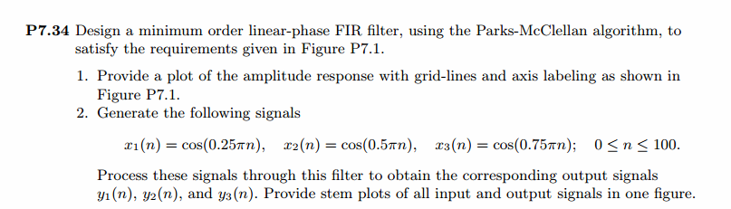
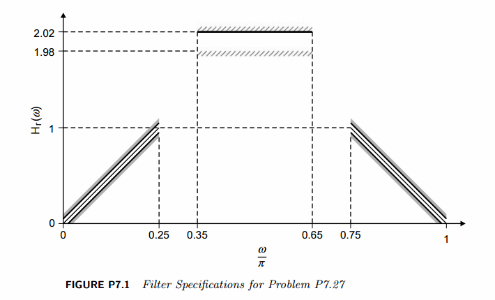
代码:
%% ++++++++++++++++++++++++++++++++++++++++++++++++++++++++++++++++++++++++++++++++

%%            Output Info about this m-file

fprintf('\n***********************************************************\n');

fprintf('        <DSP using MATLAB> Problem 7.34 \n\n');

banner();

%% ++++++++++++++++++++++++++++++++++++++++++++++++++++++++++++++++++++++++++++++++

% bandpass in Fig P7.1

ws1 = 0.25*pi; wp1 = 0.35*pi; wp2 = 0.65*pi; ws2=0.75*pi;

delta1 = 0.05; delta2 = 0.02; delta3 = 0.05;

weights = [1  delta3/delta2  1];

Dw = min((wp1-ws1), (ws2-wp2));

M = ceil((-20*log10((delta1*delta2*delta3)^(1/3)) - 13) / (2.285*Dw) + 1)

deltaH = max([delta1,delta2,delta3]); deltaL = min([delta1,delta2,delta3]);

f = [ 0  ws1 wp1 wp2 ws2  pi]/pi;

m = [ 0  1   2   2   1  0];

h = firpm(M-1, f, m, weights);

[db, mag, pha, grd, w] = freqz_m(h, [1]);

delta_w = 2*pi/1000;

ws1i = floor(ws1/delta_w)+1; wp1i = floor(wp1/delta_w)+1;

wp2i = floor(wp2/delta_w)+1; ws2i = floor(ws2/delta_w)+1;

Asd = -max(db(1:ws1i))

%[Hr, ww, a, L] = Hr_Type1(h);

[Hr,omega,P,L] = ampl_res(h);

l = 0:M-1;

%% -------------------------------------------------

%%                    Plot

%% -------------------------------------------------

figure('NumberTitle', 'off', 'Name', 'Problem 7.34 Parks-McClellan Method')

set(gcf,'Color','white');

subplot(2,2,1); stem(l, h); axis([-1, M, -0.6, 1.3]); grid on;

xlabel('n'); ylabel('h(n)'); title('Actual Impulse Response, M=23');

set(gca,'XTickMode','manual','XTick',[0,M-1])

set(gca,'YTickMode','manual','YTick',[-0.6:0.2:1.4])

subplot(2,2,2); plot(w/pi, db); axis([0, 1, -80, 10]); grid on;

xlabel('frequency in \pi units'); ylabel('Decibels'); title('Magnitude Response in dB ');

set(gca,'XTickMode','manual','XTick',f)

set(gca,'YTickMode','manual','YTick',[-60,-30,0]);

set(gca,'YTickLabelMode','manual','YTickLabel',['60';'30';' 0']);

subplot(2,2,3); plot(omega/pi, Hr); axis([0, 1, -0.2, 2.2]); grid on;

xlabel('frequency in \pi nuits'); ylabel('Hr(w)'); title('Amplitude Response');

set(gca,'XTickMode','manual','XTick',f)

set(gca,'YTickMode','manual','YTick',[0,1,1.98,2.02]);

subplot(2,2,4); axis([0, 1, -deltaH, deltaH]);

sb1w = omega(1:1:ws1i)/pi; sb1e = (Hr(1:1:ws1i)-m(1)); %sb1e = (Hr(1:1:ws1i)-m(1))*weights(1);

pbw = omega(wp1i:wp2i)/pi; pbe = (Hr(wp1i:wp2i)-m(3)); %pbe = (Hr(wp1i:wp2i)-m(3))*weights(2);

sb2w = omega(ws2i:501)/pi; sb2e = (Hr(ws2i:501)-m(5)); %sb2e = (Hr(ws2i:501)-m(5))*weights(3);

plot(sb1w,sb1e,pbw,pbe,sb2w,sb2e); grid on;

xlabel('frequency in \pi units'); ylabel('Hr(w)'); title('Error Response'); %title('Weighted Error');

set(gca,'XTickMode','manual','XTick',f);

%set(gca,'YTickMode','manual','YTick',[-deltaH,0,deltaH]);

figure('NumberTitle', 'off', 'Name', 'Problem 7.34 AmpRes of h(n), Parks-McClellan Method')

set(gcf,'Color','white');

plot(omega/pi, Hr); grid on; %axis([0 1 -100 10]);

xlabel('frequency in \pi units'); ylabel('Hr'); title('Amplitude Response');

set(gca,'YTickMode','manual','YTick',[0, 1, 1.98, 2.02]);

%set(gca,'YTickLabelMode','manual','YTickLabel',['90';'40';' 0']);

set(gca,'XTickMode','manual','XTick',[0,0.25,0.35,0.65,0.75,1]);

%% -------------------------------------------------------

%%       Input is given, and we want the Output

%% -------------------------------------------------------

num = 100;

n_x1 = [0:1:num]; x1 = cos(0.25*pi*n_x1);

n_x2 = n_x1; x2 = cos(0.5*pi*n_x2);

n_x3 = n_x1; x3 = cos(0.75*pi*n_x3);

% Output

y1 = filter(h, 1, x1);

n_y1 = n_x1;

y2 = filter(h, 1, x2);

n_y2 = n_x2;

y3 = filter(h, 1, x3);

n_y3 = n_x3;

figure('NumberTitle', 'off', 'Name', 'Problem 7.34 Input[x1(n)] and Output[y1(n)]');

set(gcf,'Color','white');

subplot(2,1,1); stem(n_x1, x1); axis([-1, 100, -1.2, 1.2]); grid on;

xlabel('n'); ylabel('x1(n)'); title('Input Response, Length=100');

subplot(2,1,2); stem(n_y1, y1); axis([-1, 100, -2, 2]); grid on;

xlabel('n'); ylabel('y1(n)'); title('Output Response');

figure('NumberTitle', 'off', 'Name', 'Problem 7.34 Input[x2(n)] and Output[y2(n)]');

set(gcf,'Color','white');

subplot(2,1,1); stem(n_x2, x2); axis([-1, 100, -1.2, 1.2]); grid on;

xlabel('n'); ylabel('x2(n)'); title('Input Response, Length=100');

subplot(2,1,2); stem(n_y2, y2); axis([-1, 100, -3, 3]); grid on;

xlabel('n'); ylabel('y2(n)'); title('Output Response');

figure('NumberTitle', 'off', 'Name', 'Problem 7.34 Input[x3(n)] and Output[y3(n)]');

set(gcf,'Color','white');

subplot(2,1,1); stem(n_x3, x3); axis([-1, 100, -1.2, 1.2]); grid on;

xlabel('n'); ylabel('x3(n)'); title('Input Response, Length=100');

subplot(2,1,2); stem(n_y3, y3); axis([-1, 100, -2, 2]); grid on;

xlabel('n'); ylabel('y3(n)'); title('Output Response');

% ---------------------------

%    DTFT of x and y

% ---------------------------

MM = 500;

[X1, w1] = dtft1(x1, n_x1, MM);

[Y1, w1] = dtft1(y1, n_y1, MM);

[X2, w1] = dtft1(x2, n_x2, MM);

[Y2, w1] = dtft1(y2, n_y2, MM);

[X3, w1] = dtft1(x3, n_x3, MM);

[Y3, w1] = dtft1(y3, n_y3, MM);

magX1 = abs(X1); angX1 = angle(X1); realX1 = real(X1); imagX1 = imag(X1);

magY1 = abs(Y1); angY1 = angle(Y1); realY1 = real(Y1); imagY1 = imag(Y1);

magX2 = abs(X2); angX2 = angle(X2); realX2 = real(X2); imagX2 = imag(X2);

magY2 = abs(Y2); angY2 = angle(Y2); realY2 = real(Y2); imagY2 = imag(Y2);

magX3 = abs(X3); angX3 = angle(X3); realX3 = real(X3); imagX3 = imag(X3);

magY3 = abs(Y3); angY3 = angle(Y3); realY3 = real(Y3); imagY3 = imag(Y3);

figure('NumberTitle', 'off', 'Name', 'Problem 7.34 DTFT of Input[x1(n)]')

set(gcf,'Color','white');

subplot(2,2,1); plot(w1/pi,magX1); grid on; %axis([0,2,0,15]);

title('Magnitude Part');

xlabel('frequency in \pi units'); ylabel('Magnitude  |X|');

subplot(2,2,3); plot(w1/pi, angX1/pi); grid on; axis([0,2,-1,1]);

title('Angle Part');

xlabel('frequency in \pi units'); ylabel('Radians/\pi');

subplot(2,2,2); plot(w1/pi, realX1); grid on;

title('Real Part');

xlabel('frequency in \pi units'); ylabel('Real');

subplot(2,2,4); plot(w1/pi, imagX1); grid on;

title('Imaginary Part');

xlabel('frequency in \pi units'); ylabel('Imaginary');

figure('NumberTitle', 'off', 'Name', 'Problem 7.34 DTFT of Output[y1(n)]')

set(gcf,'Color','white');

subplot(2,2,1); plot(w1/pi,magY1); grid on; %axis([0,2,0,15]);

title('Magnitude Part');

xlabel('frequency in \pi units'); ylabel('Magnitude  |Y|');

subplot(2,2,3); plot(w1/pi, angY1/pi); grid on; axis([0,2,-1,1]);

title('Angle Part');

xlabel('frequency in \pi units'); ylabel('Radians/\pi');

subplot(2,2,2); plot(w1/pi, realY1); grid on;

title('Real Part');

xlabel('frequency in \pi units'); ylabel('Real');

subplot(2,2,4); plot(w1/pi, imagY1); grid on;

title('Imaginary Part');

xlabel('frequency in \pi units'); ylabel('Imaginary');

figure('NumberTitle', 'off', 'Name', 'Problem 7.34 Magnitude Response')

set(gcf,'Color','white');

subplot(1,2,1); plot(w1/pi,magX1); grid on; %axis([0,2,0,15]);

title('Magnitude Part of Input');

xlabel('frequency in \pi units'); ylabel('Magnitude  |X|');

subplot(1,2,2); plot(w1/pi,magY1); grid on; %axis([0,2,0,15]);

title('Magnitude Part of Output');

xlabel('frequency in \pi units'); ylabel('Magnitude  |Y|');

figure('NumberTitle', 'off', 'Name', 'Problem 7.34 DTFT of Input[x2(n)]')

set(gcf,'Color','white');

subplot(2,2,1); plot(w1/pi,magX2); grid on; %axis([0,2,0,15]);

title('Magnitude Part');

xlabel('frequency in \pi units'); ylabel('Magnitude  |X|');

subplot(2,2,3); plot(w1/pi, angX2/pi); grid on; axis([0,2,-1,1]);

title('Angle Part');

xlabel('frequency in \pi units'); ylabel('Radians/\pi');

subplot(2,2,2); plot(w1/pi, realX2); grid on;

title('Real Part');

xlabel('frequency in \pi units'); ylabel('Real');

subplot(2,2,4); plot(w1/pi, imagX2); grid on;

title('Imaginary Part');

xlabel('frequency in \pi units'); ylabel('Imaginary');

figure('NumberTitle', 'off', 'Name', 'Problem 7.34 DTFT of Output[y2(n)]')

set(gcf,'Color','white');

subplot(2,2,1); plot(w1/pi,magY2); grid on; %axis([0,2,0,15]);

title('Magnitude Part');

xlabel('frequency in \pi units'); ylabel('Magnitude  |Y|');

subplot(2,2,3); plot(w1/pi, angY2/pi); grid on; axis([0,2,-1,1]);

title('Angle Part');

xlabel('frequency in \pi units'); ylabel('Radians/\pi');

subplot(2,2,2); plot(w1/pi, realY2); grid on;

title('Real Part');

xlabel('frequency in \pi units'); ylabel('Real');

subplot(2,2,4); plot(w1/pi, imagY2); grid on;

title('Imaginary Part');

xlabel('frequency in \pi units'); ylabel('Imaginary');

figure('NumberTitle', 'off', 'Name', 'Problem 7.34 Magnitude Response')

set(gcf,'Color','white');

subplot(1,2,1); plot(w1/pi,magX2); grid on; %axis([0,2,0,15]);

title('Magnitude Part of Input');

xlabel('frequency in \pi units'); ylabel('Magnitude  |X|');

subplot(1,2,2); plot(w1/pi,magY2); grid on; %axis([0,2,0,15]);

title('Magnitude Part of Output');

xlabel('frequency in \pi units'); ylabel('Magnitude  |Y|');

figure('NumberTitle', 'off', 'Name', 'Problem 7.34 DTFT of Input[x3(n)]')

set(gcf,'Color','white');

subplot(2,2,1); plot(w1/pi,magX3); grid on; %axis([0,2,0,15]);

title('Magnitude Part');

xlabel('frequency in \pi units'); ylabel('Magnitude  |X|');

subplot(2,2,3); plot(w1/pi, angX3/pi); grid on; axis([0,2,-1,1]);

title('Angle Part');

xlabel('frequency in \pi units'); ylabel('Radians/\pi');

subplot(2,2,2); plot(w1/pi, realX3); grid on;

title('Real Part');

xlabel('frequency in \pi units'); ylabel('Real');

subplot(2,2,4); plot(w1/pi, imagX3); grid on;

title('Imaginary Part');

xlabel('frequency in \pi units'); ylabel('Imaginary');

figure('NumberTitle', 'off', 'Name', 'Problem 7.34 DTFT of Output[y3(n)]')

set(gcf,'Color','white');

subplot(2,2,1); plot(w1/pi,magY3); grid on; %axis([0,2,0,15]);

title('Magnitude Part');

xlabel('frequency in \pi units'); ylabel('Magnitude  |Y|');

subplot(2,2,3); plot(w1/pi, angY3/pi); grid on; axis([0,2,-1,1]);

title('Angle Part');

xlabel('frequency in \pi units'); ylabel('Radians/\pi');

subplot(2,2,2); plot(w1/pi, realY3); grid on;

title('Real Part');

xlabel('frequency in \pi units'); ylabel('Real');

subplot(2,2,4); plot(w1/pi, imagY3); grid on;

title('Imaginary Part');

xlabel('frequency in \pi units'); ylabel('Imaginary');

figure('NumberTitle', 'off', 'Name', 'Problem 7.34 Magnitude Response')

set(gcf,'Color','white');

subplot(1,2,1); plot(w1/pi,magX3); grid on; %axis([0,2,0,15]);

title('Magnitude Part of Input');

xlabel('frequency in \pi units'); ylabel('Magnitude  |X|');

subplot(1,2,2); plot(w1/pi,magY3); grid on; %axis([0,2,0,15]);

title('Magnitude Part of Output');

xlabel('frequency in \pi units'); ylabel('Magnitude  |Y|');
运行结果:
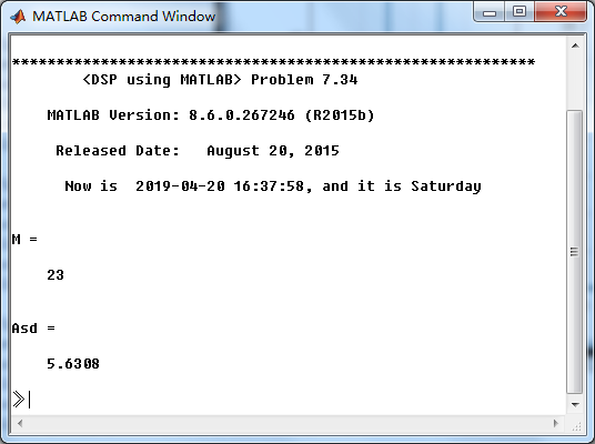
用P-M法设计出来滤波器长度M=23
幅度谱如下

振幅谱如下:

第2个输入,及对应的输出
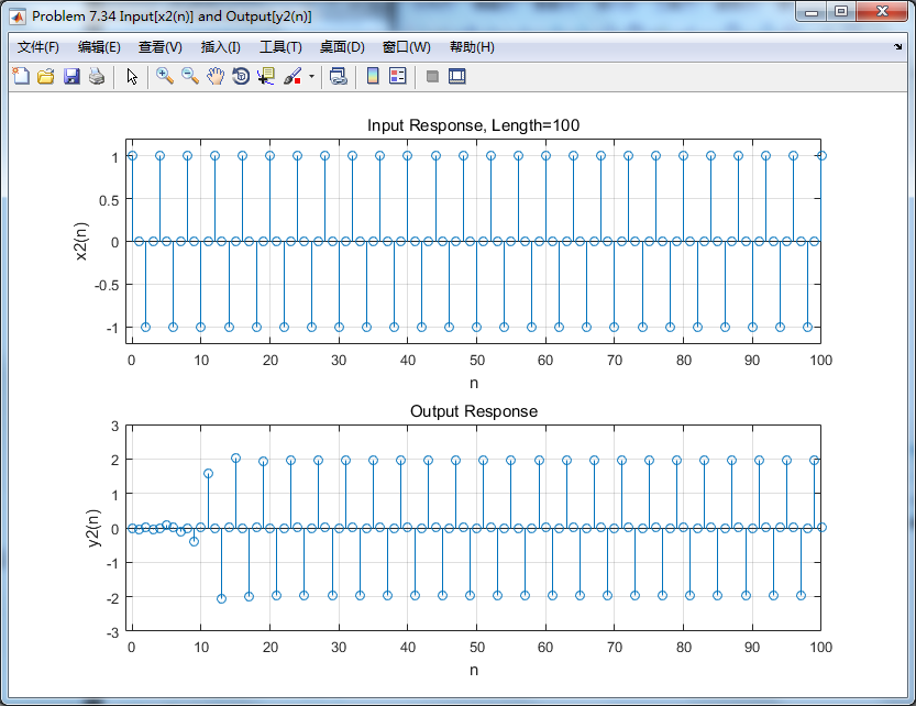
第2个输入输出的谱(DTFT)对比:
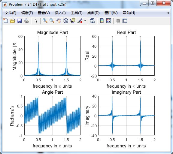
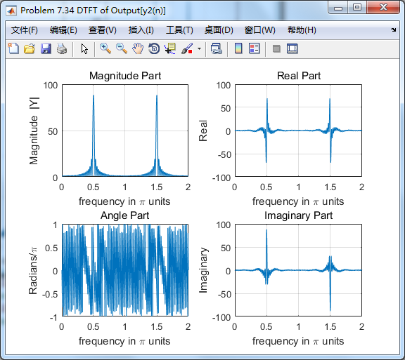

从图中看,输入0.5π分量幅度有所增大,几乎达到原来的2倍。
《DSP using MATLAB》Problem 7.34的更多相关文章
- 《DSP using MATLAB》Problem 5.34
第1小题 代码: %% ++++++++++++++++++++++++++++++++++++++++++++++++++++++++++++++++++++++++++++++++++++++++ ...
- 《DSP using MATLAB》Problem 8.34
今天下了小雨,空气中泛起潮湿的味道,阴冷的感觉袭来,心情受到小小影响. 代码: hp2lpfre子函数 function [wpLP, wsLP, alpha] = hp2lpfre(wphp, ws ...
- 《DSP using MATLAB》Problem 7.12
阻带衰减50dB,我们选Hamming窗 代码: %% ++++++++++++++++++++++++++++++++++++++++++++++++++++++++++++++++++++++++ ...
- 《DSP using MATLAB》Problem 7.35
代码: %% ++++++++++++++++++++++++++++++++++++++++++++++++++++++++++++++++++++++++++++++++ %% Output In ...
- 《DSP using MATLAB》Problem 7.27
代码: %% ++++++++++++++++++++++++++++++++++++++++++++++++++++++++++++++++++++++++++++++++ %% Output In ...
- 《DSP using MATLAB》Problem 7.26
注意:高通的线性相位FIR滤波器,不能是第2类,所以其长度必须为奇数.这里取M=31,过渡带里采样值抄书上的. 代码: %% +++++++++++++++++++++++++++++++++++++ ...
- 《DSP using MATLAB》Problem 7.25
代码: %% ++++++++++++++++++++++++++++++++++++++++++++++++++++++++++++++++++++++++++++++++ %% Output In ...
- 《DSP using MATLAB》Problem 7.24
又到清明时节,…… 注意:带阻滤波器不能用第2类线性相位滤波器实现,我们采用第1类,长度为基数,选M=61 代码: %% +++++++++++++++++++++++++++++++++++++++ ...
- 《DSP using MATLAB》Problem 7.23
%% ++++++++++++++++++++++++++++++++++++++++++++++++++++++++++++++++++++++++++++++++ %% Output Info a ...
随机推荐
- Python flask 构建微电影视频网站✍✍✍
Python flask 构建微电影视频网站 整个课程都看完了,这个课程的分享可以往下看,下面有链接,之前做java开发也做了一些年头,也分享下自己看这个视频的感受,单论单个知识点课程本身没问题,大 ...
- <随便写>同步,异步进程池,线程
from multiprocessing import Pool import time import os def work(n): print("%s run" % os.ge ...
- MVC中利用ViewBag传递Json数据时的前端处理方法
用viewBag传递Json字符串到前端时,json字符串中的“会被转义为& quot,前端处理方法为@Html.Raw(Json.Encode(ViewBag.Data)),再用eval() ...
- 2019-8-31-dotnet-获取指定进程的输入命令行
title author date CreateTime categories dotnet 获取指定进程的输入命令行 lindexi 2019-08-31 16:55:58 +0800 2019-0 ...
- JS规则 自加一,自减一 ( ++和- -) 【mynum = mynum + 1;//等同于mynum++;】
自加一,自减一 ( ++和- -) 算术操作符除了(+.-.*./)外,还有两个非常常用的操作符,自加一"++":自减一"--".首先来看一个例子: mynum ...
- Pascal代码自动格式化
const WEnter=; key=; next_line:..WEnter]of string=(';','begin','else','then','repeat','do','var'); k ...
- 函数的作用域、作用域链以及return关键字
1.作用域 全局作用域:在函数外部使用var关键字定义的变量 局部作用域:在函数内部使用var关键字定义的变量 特点 (1)局部变量无法直接影响全局变量 (2)在局部作用域中可以使用全局作用 ...
- linux 服务 启动 关闭 列表
##查看服务在每个级别的运行状态 chkconfig --list httpd 0:关闭 1:关闭 2:关闭 3:关闭 4:关闭 5:启用 6:关闭 bluetooth ...
- gulp 前端构建工具使用
gulp 前端构建工具使用 1.新建一个web h5项目 2.准备好gulpfile.js文件 (1)下载链接:https://pan.baidu.com/s/116J-BaYOMRzeJW3i_J ...
- Python学习day05 - Python基础(3) 格式化输出和基本运算符
figure:last-child { margin-bottom: 0.5rem; } #write ol, #write ul { position: relative; } img { max- ...