吴裕雄--天生自然 R语言开发学习：使用ggplot2进行高级绘图（续二）

#----------------------------------------------------------#
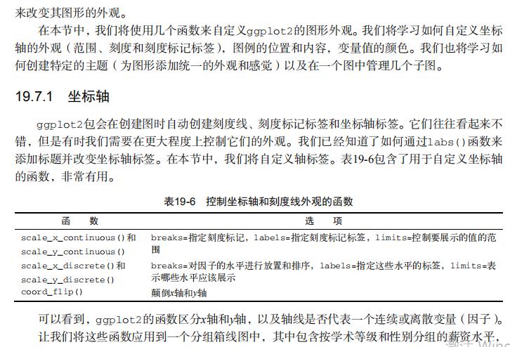
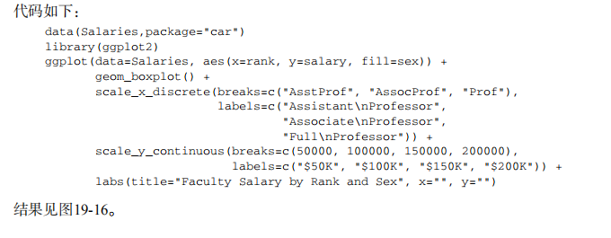
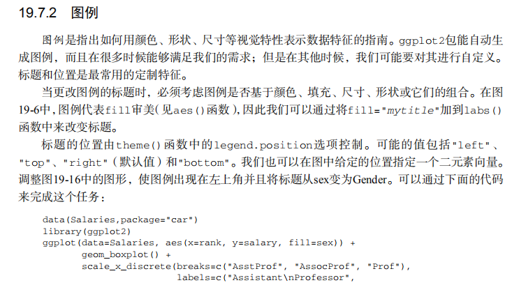
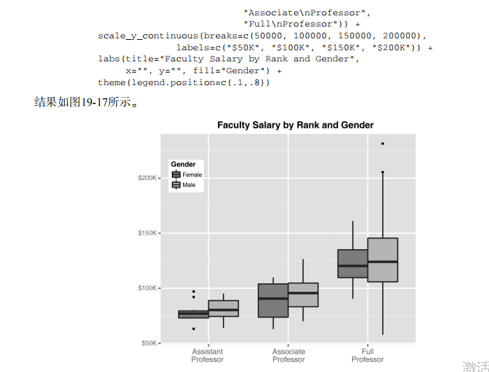
# R in Action (2nd ed): Chapter 19                         #
# Advanced graphics with ggplot2                           #
# requires packages ggplot2, RColorBrewer, gridExtra,      #
#   and car (for datasets)                                 #
# install.packages(c("ggplot2", "gridExtra",               #
#      "RColorBrewer", "car"))                             #
#----------------------------------------------------------#

par(ask=TRUE)

# Basic scatterplot
library(ggplot2)
ggplot(data=mtcars, aes(x=wt, y=mpg)) +
  geom_point() +
  labs(title="Automobile Data", x="Weight", y="Miles Per Gallon")

# Scatter plot with additional options
library(ggplot2)
ggplot(data=mtcars, aes(x=wt, y=mpg)) +
  geom_point(pch=17, color="blue", size=2) +
  geom_smooth(method="lm", color="red", linetype=2) +
  labs(title="Automobile Data", x="Weight", y="Miles Per Gallon")

# Scatter plot with faceting and grouping
data(mtcars)
mtcars$am <- factor(mtcars$am, levels=c(0,1),
                    labels=c("Automatic", "Manual"))
mtcars$vs <- factor(mtcars$vs, levels=c(0,1),
                    labels=c("V-Engine", "Straight Engine"))
mtcars$cyl <- factor(mtcars$cyl)

library(ggplot2)
ggplot(data=mtcars, aes(x=hp, y=mpg,
                        shape=cyl, color=cyl)) +
  geom_point(size=3) +
  facet_grid(am~vs) +
  labs(title="Automobile Data by Engine Type",
       x="Horsepower", y="Miles Per Gallon")

# Using geoms
data(singer, package="lattice")
ggplot(singer, aes(x=height)) + geom_histogram()

ggplot(singer, aes(x=voice.part, y=height)) + geom_boxplot()

data(Salaries, package="car")
library(ggplot2)
ggplot(Salaries, aes(x=rank, y=salary)) +
  geom_boxplot(fill="cornflowerblue",
               color="black", notch=TRUE)+
  geom_point(position="jitter", color="blue", alpha=.5)+
  geom_rug(side="l", color="black")

# Grouping
library(ggplot2)
data(singer, package="lattice")
ggplot(singer, aes(x=voice.part, y=height)) +
  geom_violin(fill="lightblue") +
  geom_boxplot(fill="lightgreen", width=.2)

data(Salaries, package="car")
library(ggplot2)
ggplot(data=Salaries, aes(x=salary, fill=rank)) +
  geom_density(alpha=.3)

ggplot(Salaries, aes(x=yrs.since.phd, y=salary, color=rank,
                     shape=sex)) + geom_point()

ggplot(Salaries, aes(x=rank, fill=sex)) +
  geom_bar(position="stack") + labs(title='position="stack"')

ggplot(Salaries, aes(x=rank, fill=sex)) +
  geom_bar(position="dodge") + labs(title='position="dodge"')

ggplot(Salaries, aes(x=rank, fill=sex)) +
  geom_bar(position="fill") + labs(title='position="fill"')

# Placing options
ggplot(Salaries, aes(x=rank, fill=sex))+ geom_bar()

ggplot(Salaries, aes(x=rank)) + geom_bar(fill="red")

ggplot(Salaries, aes(x=rank, fill="red")) + geom_bar()

# Faceting
data(singer, package="lattice")
library(ggplot2)
ggplot(data=singer, aes(x=height)) +
  geom_histogram() +
  facet_wrap(~voice.part, nrow=4)

library(ggplot2)
ggplot(Salaries, aes(x=yrs.since.phd, y=salary, color=rank,
                     shape=rank)) + geom_point() + facet_grid(.~sex)

data(singer, package="lattice")
library(ggplot2)
ggplot(data=singer, aes(x=height, fill=voice.part)) +
  geom_density() +
  facet_grid(voice.part~.)

# Adding smoothed lines
data(Salaries, package="car")
library(ggplot2)
ggplot(data=Salaries, aes(x=yrs.since.phd, y=salary)) +
  geom_smooth() + geom_point()

ggplot(data=Salaries, aes(x=yrs.since.phd, y=salary,
                          linetype=sex, shape=sex, color=sex)) +
  geom_smooth(method=lm, formula=y~poly(x,2),
              se=FALSE, size=1) +
  geom_point(size=2)

# Modifying axes
data(Salaries,package="car")
library(ggplot2)
ggplot(data=Salaries, aes(x=rank, y=salary, fill=sex)) +
  geom_boxplot() +
  scale_x_discrete(breaks=c("AsstProf", "AssocProf", "Prof"),
                   labels=c("Assistant\nProfessor",
                            "Associate\nProfessor",
                            "Full\nProfessor")) +
  scale_y_continuous(breaks=c(50000, 100000, 150000, 200000),
                     labels=c("$50K", "$100K", "$150K", "$200K")) +
  labs(title="Faculty Salary by Rank and Sex", x="", y="")

# Legends
data(Salaries,package="car")
library(ggplot2)
ggplot(data=Salaries, aes(x=rank, y=salary, fill=sex)) +
  geom_boxplot() +
  scale_x_discrete(breaks=c("AsstProf", "AssocProf", "Prof"),
                   labels=c("Assistant\nProfessor",
                            "Associate\nProfessor",
                            "Full\nProfessor")) +
  scale_y_continuous(breaks=c(50000, 100000, 150000, 200000),
                     labels=c("$50K", "$100K", "$150K", "$200K")) +
  labs(title="Faculty Salary by Rank and Gender",
       x="", y="", fill="Gender") +
  theme(legend.position=c(.1,.8))

# Scales
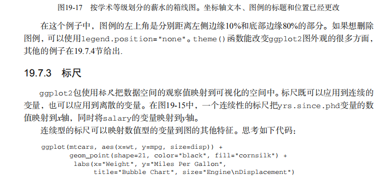
ggplot(mtcars, aes(x=wt, y=mpg, size=disp)) +
  geom_point(shape=21, color="black", fill="cornsilk") +
  labs(x="Weight", y="Miles Per Gallon",
       title="Bubble Chart", size="Engine\nDisplacement")

data(Salaries, package="car")
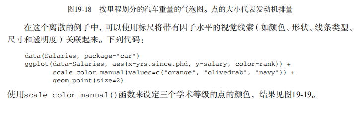
ggplot(data=Salaries, aes(x=yrs.since.phd, y=salary, color=rank)) +
  scale_color_manual(values=c("orange", "olivedrab", "navy")) +
  geom_point(size=2)

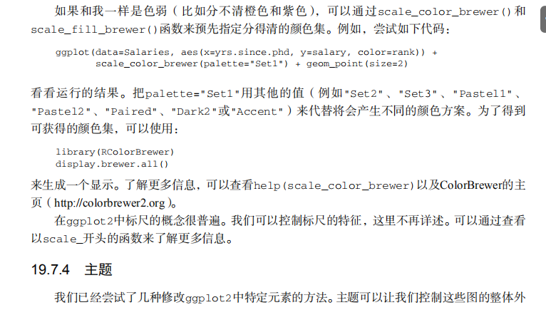
ggplot(data=Salaries, aes(x=yrs.since.phd, y=salary, color=rank)) +
  scale_color_brewer(palette="Set1") + geom_point(size=2)

library(RColorBrewer)
display.brewer.all()

# Themes
data(Salaries, package="car")
library(ggplot2)
mytheme <- theme(plot.title=element_text(face="bold.italic",
                                         size="", color="brown"),
                 axis.title=element_text(face="bold.italic",
                                         size=10, color="brown"),
                 axis.text=element_text(face="bold", size=9,
                                        color="darkblue"),
                 panel.background=element_rect(fill="white",
                                               color="darkblue"),
                 panel.grid.major.y=element_line(color="grey",
                                                 linetype=1),
                 panel.grid.minor.y=element_line(color="grey",
                                                 linetype=2),
                 panel.grid.minor.x=element_blank(),
                 legend.position="top")

ggplot(Salaries, aes(x=rank, y=salary, fill=sex)) +
  geom_boxplot() +
  labs(title="Salary by Rank and Sex",
       x="Rank", y="Salary") +
  mytheme

# Multiple graphs per page
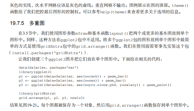
data(Salaries, package="car")
library(ggplot2)
p1 <- ggplot(data=Salaries, aes(x=rank)) + geom_bar()
p2 <- ggplot(data=Salaries, aes(x=sex)) + geom_bar()
p3 <- ggplot(data=Salaries, aes(x=yrs.since.phd, y=salary)) + geom_point()

library(gridExtra)
grid.arrange(p1, p2, p3, ncol=3)

# Saving graphs
ggplot(data=mtcars, aes(x=mpg)) + geom_histogram()
ggsave(file="mygraph.pdf")