《DSP using MATLAB》Problem 8.30
10月1日,新中国70周岁生日,上午观看了盛大的庆祝仪式,整齐的方阵,先进的武器,尊敬的先辈英雄,欢乐的人们,愿我们的
国家越来越好,人民生活越来越好。
接着做题。
代码:
%% ------------------------------------------------------------------------
%% Output Info about this m-file
fprintf('\n***********************************************************\n');
fprintf(' <DSP using MATLAB> Problem 8.30 \n\n'); banner();
%% ------------------------------------------------------------------------ % -----------------------------------
% Ω=(2/T)tan(ω/2)
% ω=2*[atan(ΩT/2)]
% Digital Filter Specifications:
% -----------------------------------
wp = 0.4*pi; % digital passband freq in rad
ws = 0.6*pi; % digital stopband freq in rad
Rp = 0.5; % passband ripple in dB
As = 50; % stopband attenuation in dB Ripple = 10 ^ (-Rp/20) % passband ripple in absolute
Attn = 10 ^ (-As/20) % stopband attenuation in absolute % Analog prototype specifications: Inverse Mapping for frequencies
T = 2; % set T = 1
Fs = 1/T;
OmegaP = (2/T)*tan(wp/2); % prototype passband freq
OmegaS = (2/T)*tan(ws/2); % prototype stopband freq % Analog Butterworth Prototype Filter Calculation:
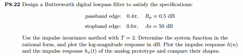
[cs, ds] = afd_butt(OmegaP, OmegaS, Rp, As); % Calculation of second-order sections:
fprintf('\n***** Cascade-form in s-plane: START *****\n');
[CS, BS, AS] = sdir2cas(cs, ds);
fprintf('\n***** Cascade-form in s-plane: END *****\n'); % Calculation of Frequency Response:
[db_s, mag_s, pha_s, ww_s] = freqs_m(cs, ds, 2*pi/T); % --------------------------------------------------------------------
% find exact band-edge frequencies for the given dB specifications
% --------------------------------------------------------------------
%ind = find( abs(ceil(db_s))-50 == 0 )
[diff_to_50dB, ind] = min(abs(db_s+50))
db_s(ind-3 : ind+3) % magnitude response, dB ww_s(ind)/(pi) % analog frequency in kpi units
%ww_s(ind)/(2*pi) % analog frequency in Hz units [sA,index] = sort(abs(db_s+50));
AA_dB = db_s(index(1:8))
AB_rad = ww_s(index(1:8))/(pi)
AC_Hz = ww_s(index(1:8))/(2*pi)
% ------------------------------------------------------------------- % Calculation of Impulse Response:
[ha, x, t] = impulse(cs, ds); % Impulse Invariance Transformation:
%[b, a] = imp_invr(cs, ds, T); % Bilinear Transformation
[b, a] = bilinear(cs, ds, Fs);
[C, B, A] = dir2cas(b, a); % Calculation of Frequency Response:
[db, mag, pha, grd, ww] = freqz_m(b, a); % --------------------------------------------------------------------
% find exact band-edge frequencies for the given dB specifications
% --------------------------------------------------------------------
%ind = find( abs(ceil(db))-50 == 0 )
[diff_to_80dB, ind] = min(abs(db+50))
db(ind-3 : ind+3) % magnitude response, dB ww(ind)/(pi)
%ww(ind)*Fs/(2*pi) (2/T)*tan(ww(ind)/2)/pi [sA,index] = sort(abs(db+50));
AA_dB = db(index(1:8))'
AB_rad = ww(index(1:8))'/pi
AC_Hz = (2/T)*tan(ww(index(1:8))'/2)/pi
% ------------------------------------------------------------------- %% -----------------------------------------------------------------
%% Plot
%% -----------------------------------------------------------------
figure('NumberTitle', 'off', 'Name', 'Problem 8.30 Analog Butterworth lowpass')
set(gcf,'Color','white');
M = 1; % Omega max subplot(2,2,1); plot(ww_s/pi, mag_s); grid on; axis([-M, M, 0, 1.2]);
xlabel(' Analog frequency in \pi units'); ylabel('|H|'); title('Magnitude in Absolute');
%set(gca, 'XTickMode', 'manual', 'XTick', [-0.876, -0.463, 0, 0.463, 0.876]); % T=1
set(gca, 'XTickMode', 'manual', 'XTick', [-0.44, -0.23, 0, 0.23, 0.44]); % T=2
set(gca, 'YTickMode', 'manual', 'YTick', [0, 0.0032, 0.5, 0.9441, 1]); subplot(2,2,2); plot(ww_s/pi, db_s); grid on; axis([-M, M, -100, 10]);
xlabel('Analog frequency in \pi units'); ylabel('Decibels'); title('Magnitude in dB ');
%set(gca, 'XTickMode', 'manual', 'XTick', [-0.876, -0.463, 0, 0.463, 0.8591, 0.876]); % T=1
set(gca, 'XTickMode', 'manual', 'XTick', [-0.44, -0.23, 0, 0.23, 0.4295, 0.44]); % T=2
set(gca, 'YTickMode', 'manual', 'YTick', [-90, -50, -1, 0]);
set(gca,'YTickLabelMode','manual','YTickLabel',['90';'50';' 1';' 0']); subplot(2,2,3); plot(ww_s/pi, pha_s/pi); grid on; axis([-M, M, -1.2, 1.2]);
xlabel('Analog frequency in \pi nuits'); ylabel('radians'); title('Phase Response');
set(gca, 'XTickMode', 'manual', 'XTick', [-OmegaS, -OmegaP, 0, OmegaP, OmegaS]/pi);
set(gca, 'YTickMode', 'manual', 'YTick', [-1:0.5:1]); subplot(2,2,4); plot(t, ha); grid on; %axis([0, 30, -0.05, 0.25]);
xlabel('time in seconds'); ylabel('ha(t)'); title('Impulse Response'); figure('NumberTitle', 'off', 'Name', 'Problem 8.30 Digital Butterworth lowpass by afd_butt function')
set(gcf,'Color','white');
M = 2; % Omega max subplot(2,2,1); plot(ww/(pi), mag); axis([0, M, 0, 1.2]); grid on;
xlabel('Digital frequency in \pi units'); ylabel('|H|'); title('Magnitude Response');
set(gca, 'XTickMode', 'manual', 'XTick', [0, 0.4, 0.6, 1.0, M]);
set(gca, 'YTickMode', 'manual', 'YTick', [0, 0.0032, 0.5, 0.9441, 1]); subplot(2,2,2); plot(ww/(pi), pha/pi); axis([0, M, -1.1, 1.1]); grid on;
xlabel('Digital frequency in \pi nuits'); ylabel('radians in \pi units'); title('Phase Response');
set(gca, 'XTickMode', 'manual', 'XTick', [0, 0.4, 0.6, 1.0, M]);
set(gca, 'YTickMode', 'manual', 'YTick', [-1:1:1]); subplot(2,2,3); plot(ww/pi, db); axis([0, M, -100, 10]); grid on;
xlabel('Digital frequency in \pi units'); ylabel('Decibels'); title('Magnitude in dB ');
%set(gca, 'XTickMode', 'manual', 'XTick', [0, 0.4, 0.594, 0.6, 1.0, M]); % T=1
set(gca, 'XTickMode', 'manual', 'XTick', [0, 0.4, 0.594, 0.6, 1.0, M]); % T=2
set(gca, 'YTickMode', 'manual', 'YTick', [-70, -50, -1, 0]);
set(gca,'YTickLabelMode','manual','YTickLabel',['70';'50';' 1';' 0']); subplot(2,2,4); plot(ww/pi, grd); grid on; %axis([0, M, 0, 35]);
xlabel('Digital frequency in \pi units'); ylabel('Samples'); title('Group Delay');
set(gca, 'XTickMode', 'manual', 'XTick', [0, 0.4, 0.6, 1.0, M]);
%set(gca, 'YTickMode', 'manual', 'YTick', [0:5:35]); figure('NumberTitle', 'off', 'Name', 'Problem 8.30 Pole-Zero Plot')
set(gcf,'Color','white');
zplane(b,a);
title(sprintf('Pole-Zero Plot'));
%pzplotz(b,a); % ----------------------------------------------
% Calculation of Impulse Response
% ----------------------------------------------
figure('NumberTitle', 'off', 'Name', 'Problem 8.30 Imp & Freq Response')
set(gcf,'Color','white');
t = [0:0.5:60]; subplot(2,1,1); impulse(cs,ds,t); grid on; % Impulse response of the analog filter
axis([0,60,-0.3,0.5]);hold on n = [0:1:60/T]; hn = filter(b,a,impseq(0,0,60/T)); % Impulse response of the digital filter
stem(n*T,hn); xlabel('time in sec'); title (sprintf('Impulse Responses, T=%f',T));
hold off % Calculation of Frequency Response:
[dbs, mags, phas, wws] = freqs_m(cs, ds, 2*pi/T); % Analog frequency s-domain [dbz, magz, phaz, grdz, wwz] = freqz_m(b, a); % Digital z-domain %% -----------------------------------------------------------------
%% Plot
%% ----------------------------------------------------------------- subplot(2,1,2); plot(wws/(2*pi), mags*Fs,'b+', wwz/(2*pi)*Fs, magz,'r'); grid on; xlabel('frequency in Hz'); title('Magnitude Responses'); ylabel('Magnitude'); text(-0.3,0.15,'Analog filter', 'Color', 'b'); text(0.4,0.55,'Digital filter', 'Color', 'r'); %% +++++++++++++++++++++++++++++++++++++++++++++++++++++++++++++++++++++
%% MATLAB butter function
%% +++++++++++++++++++++++++++++++++++++++++++++++++++++++++++++++++++++
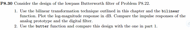
% Analog Prototype Order Calculations:
N = ceil((log10((10^(Rp/10)-1)/(10^(As/10)-1)))/(2*log10(OmegaP/OmegaS)));
fprintf('\n\n ********** Butterworth Filter Order = %3.0f \n', N) OmegaC = OmegaP/((10^(Rp/10)-1)^(1/(2*N))); % Analog BW prototype cutoff freq
wn = 2*atan((OmegaC*T)/2); % Digital BW cutoff freq % Digital Butterworth Filter Design:
wn = wn/pi; % Digital Butterworth cutoff freq in pi units [b, a] = butter(N, wn); [C, B, A] = dir2cas(b, a) % Calculation of Frequency Response:
[db, mag, pha, grd, ww] = freqz_m(b, a); figure('NumberTitle', 'off', 'Name', 'Problem 8.30 Digital Butterworth lowpass by butter function')
set(gcf,'Color','white');
M = 2; % Omega max subplot(2,2,1); plot(ww/pi, mag); axis([0, M, 0, 1.2]); grid on;
xlabel(' frequency in \pi units'); ylabel('|H|'); title('Magnitude Response');
set(gca, 'XTickMode', 'manual', 'XTick', [0, 0.4, 0.6, 1.0, M]);
set(gca, 'YTickMode', 'manual', 'YTick', [0, 0.0032, 0.5, 0.9441, 1]); subplot(2,2,2); plot(ww/pi, pha/pi); axis([0, M, -1.1, 1.1]); grid on;
xlabel('frequency in \pi nuits'); ylabel('radians in \pi units'); title('Phase Response');
set(gca, 'XTickMode', 'manual', 'XTick', [0, 0.4, 0.6, 1.0, M]);
set(gca, 'YTickMode', 'manual', 'YTick', [-1:1:1]); subplot(2,2,3); plot(ww/pi, db); axis([0, M, -100, 10]); grid on;
xlabel('frequency in \pi units'); ylabel('Decibels'); title('Magnitude in dB ');
set(gca, 'XTickMode', 'manual', 'XTick', [0, 0.4, 0.6, 1.0, M]);
set(gca, 'YTickMode', 'manual', 'YTick', [-70, -50, -1, 0]);
set(gca,'YTickLabelMode','manual','YTickLabel',['70';'50';' 1';' 0']); subplot(2,2,4); plot(ww/pi, grd); grid on; %axis([0, M, 0, 35]);
xlabel('frequency in \pi units'); ylabel('Samples'); title('Group Delay');
set(gca, 'XTickMode', 'manual', 'XTick', [0, 0.4, 0.6, 1.0, M]);
%set(gca, 'YTickMode', 'manual', 'YTick', [0:5:35]); figure('NumberTitle', 'off', 'Name', 'Problem 8.30 Pole-Zero Plot')
set(gcf,'Color','white');
zplane(b,a);
title(sprintf('Pole-Zero Plot'));
%pzplotz(b,a); % ----------------------------------------------
% Calculation of Impulse Response
% ----------------------------------------------
figure('NumberTitle', 'off', 'Name', 'Problem 8.30 Imp & Freq Response')
set(gcf,'Color','white');
t = [0:0.5:60]; subplot(2,1,1); impulse(cs,ds,t); grid on; % Impulse response of the analog filter
axis([0,60,-0.3,0.5]);hold on n = [0:1:60/T]; hn = filter(b,a,impseq(0,0,60/T)); % Impulse response of the digital filter
stem(n*T,hn); xlabel('time in sec'); title (sprintf('Impulse Responses, T=%f',T));
hold off % Calculation of Frequency Response:
[dbs, mags, phas, wws] = freqs_m(cs, ds, 2*pi/T); % Analog frequency s-domain [dbz, magz, phaz, grdz, wwz] = freqz_m(b, a); % Digital z-domain %% -----------------------------------------------------------------
%% Plot
%% ----------------------------------------------------------------- subplot(2,1,2); plot(wws/(2*pi), mags*Fs,'b+', wwz/(2*pi)*Fs, magz,'r'); grid on; xlabel('frequency in Hz'); title('Magnitude Responses'); ylabel('Magnitude'); text(-0.3,0.15,'Analog filter', 'Color', 'b'); text(0.4,0.55,'Digital filter', 'Color', 'r');
运行结果:
非归一化Butterworth模拟原型低通滤波器,直接形式的系数,
模拟低通串联形式的系数:
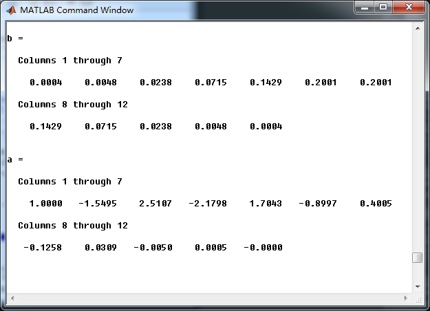
用双线性变换法,转换成数字Butterworth低通,直接形式的系数如下
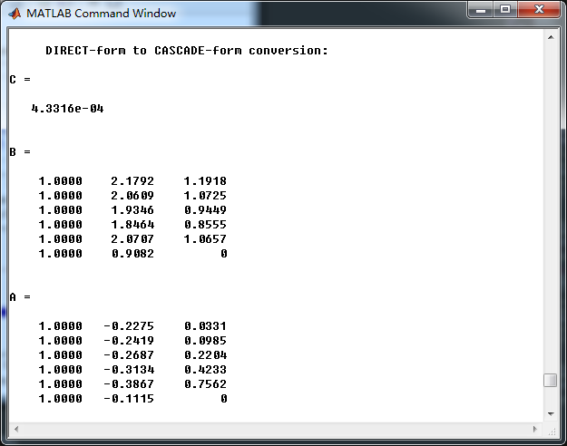
数字低通串联形式系数
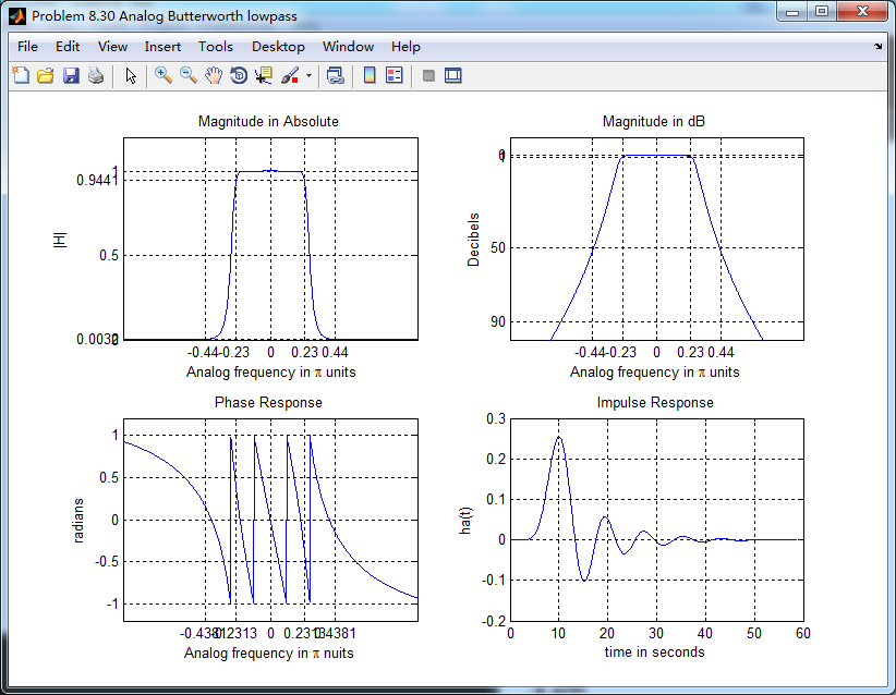
模拟Butterworth低通原型滤波器的幅度谱、相位谱和脉冲响应
双线性变换法,得到的数字Butterworth低通滤波器,起幅度谱、相位谱和群延迟响应

数字低通系统函数的零极点图

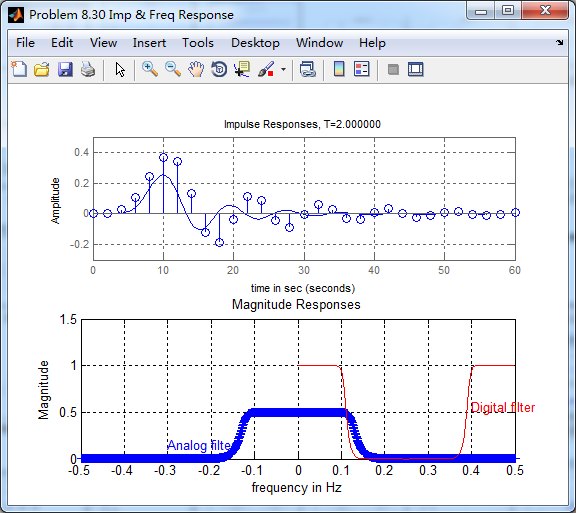
下图的上半部分,模拟低通和数字低通的脉冲响应对比,可以看出形态不一致。

采用MATLAB自带的butter函数求取数字低通,其幅度谱、相位谱和群延迟。
与上面afd_butt函数所得结果相比,相位谱和群延迟稍有不同。

零极点图,也稍有不同,零点部分靠的更紧密。

脉冲响应,与上一种方法对比,结果一样,看不出区别。
《DSP using MATLAB》Problem 8.30的更多相关文章
- 《DSP using MATLAB》Problem 7.30
代码: %% ++++++++++++++++++++++++++++++++++++++++++++++++++++++++++++++++++++++++++++++++ %% Output In ...
- 《DSP using MATLAB》Problem 5.30
代码: %% ++++++++++++++++++++++++++++++++++++++++++++++++++++++++++++++++++++++++++++++++ %% Output In ...
- 《DSP using MATLAB》Problem 7.23
%% ++++++++++++++++++++++++++++++++++++++++++++++++++++++++++++++++++++++++++++++++ %% Output Info a ...
- 《DSP using MATLAB》Problem 5.22
代码: %% ++++++++++++++++++++++++++++++++++++++++++++++++++++++++++++++++++++++++++++++++++++++++ %% O ...
- 《DSP using MATLAB》Problem 5.20
窗外的知了叽叽喳喳叫个不停,屋里温度应该有30°,伏天的日子难过啊! 频率域的方法来计算圆周移位 代码: 子函数的 function y = cirshftf(x, m, N) %% -------- ...
- 《DSP using MATLAB》Problem 3.8
2018年元旦,他乡加班中,外面尽是些放炮的,别人的繁华与我无关. 代码: %% ----------------------------------------------------------- ...
- 《DSP using MATLAB》Problem 3.3
按照题目的意思需要利用DTFT的性质,得到序列的DTFT结果(公式表示),本人数学功底太差,就不写了,直接用 书中的方法计算并画图. 代码: %% -------------------------- ...
- 《DSP using MATLAB》Problem 2.20
代码: %% ------------------------------------------------------------------------ %% Output Info about ...
- 《DSP using MATLAB》Problem 2.14
代码: %% ------------------------------------------------------------------------ %% Output Info about ...
随机推荐
- WebApi路由机制详解
随着前后端分离的大热,WebApi在项目中的作用也是越来越重要,由于公司的原因我之前一直没有机会参与前后端分离的项目,但WebApi还是要学的呀,因为这东西确实很有用,可单独部署.与前端和App交互都 ...
- How to Hide Apache Tomcat Version Number from Error Pages
1. 进入tomcat lib目录 cd /usr/local/tomcat7/lib 2. 解压catalina.jar jar xvf catalina.jar 3. 修改ServerInfo.p ...
- 1 A+B问题
原题网址: http://www.lintcode.com/zh-cn/problem/a-b-problem/# 给出两个整数a和b, 求他们的和, 但不能使用 + 等数学运算符. 注意事项 你不需 ...
- ASP.NET的底层体系2
文章引导 1.ASP.NET的底层体系1 2.ASP.NET的底层体系2 引言 接着上一篇ASP.NET的底层体系1我们继续往下走 一.System.Web.HttpRuntime.ProcessRe ...
- Astar伪代码
while(OPEN!=NULL) { 从OPEN表中取估价值f最小的节点n; if(n节点==目标节点){ break; } for(当前节点n 的每个子节点X) { 算X的估价值; if(X in ...
- Git 比较两个分支之间的差异
1.查看 dev 有,而 master 中没有的: git log dev ^master 2.查看 dev 中比 master 中多提交了哪些内容: git log master..dev 注意,列 ...
- uoj#311 【UNR #2】积劳成疾
题目 考虑直接顺着从\(1\)填数填到\(n\)发现这是在胡扯 所以考虑一些奇诡的东西,譬如最后的答案长什么样子 显然某一种方案的贡献是一个\(\prod_{i=1}^nw_i^{t_i}\)状物,\ ...
- wpf 几种常用控件样式
转自:http://blog.csdn.net/xuejiren/article/details/39449515
- wpf问题集锦
一.今天用vs2013新建wpf程序,项目名称命名为MainWindow,一启动就出现错误:类型“MainWindow.MainWindow”中不存在类型名称"App".博主顿时很 ...
- java_新特性未整理
得到的.className method.isAnnotationPresent:判断是否有指定的注解,注解.class method.invoke:执行 */}