
《DSP using MATLAB》Problem 7.36
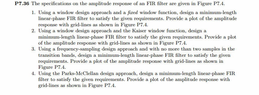
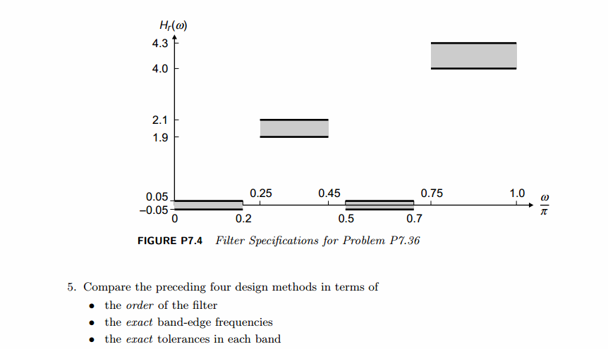
代码:
%% ++++++++++++++++++++++++++++++++++++++++++++++++++++++++++++++++++++++++++++++++

%%            Output Info about this m-file

fprintf('\n***********************************************************\n');

fprintf('        <DSP using MATLAB> Problem 7.36 \n\n');

banner();

%% ++++++++++++++++++++++++++++++++++++++++++++++++++++++++++++++++++++++++++++++++

% arbitury shape pass

w1 = 0;       w2 = 0.20*pi; delta1 = 0.05; gain1 = 0.00;

w3 = 0.25*pi; w4 = 0.45*pi; delta2 = 0.10; gain2 = 2.00;

w5 = 0.50*pi; w6 = 0.70*pi; delta3 = 0.05; gain3 = 0.00;

w7 = 0.75*pi; w8 = pi;      delta4 = 0.15; gain4 = 4.15;

fprintf('\n --- Filter Specifications START ---\n');

Rp1 = -20*log10((gain2-delta2)/(gain2+delta2))

As1 = -20*log10(delta1/(gain2+delta2))

Rp2 = -20*log10((gain4-delta4)/(gain4+delta4))

As2 = -20*log10(delta3/(gain4+delta4))

fprintf('\n --- Filter Specifications E N D ---\n');

As = min(As1, As2);

fprintf('\n --- Fix Window Method ---\n');

tr_width = min((w3-w2), (w5-w4));

%% ---------------------------------------------------

%%         1  Rectangular Window

%% ---------------------------------------------------

M = ceil(1.8*pi/tr_width) + 1;                 % Rectangular Window   M=37

M=M+190;

fprintf('\n\n#1.Rectangular Window, Filter Length M=%d.\n', M);

n = [0:1:M-1]; wc1 = (w2+w3)/2; wc2 = (w4+w5)/2; wc3 = (w6+w7)/2;

hd = 2*(ideal_lp(wc2, M) - ideal_lp(wc1, M)) + 4.15*(ideal_lp(pi, M) - ideal_lp(wc3, M));

w_rect = (boxcar(M))';  h = hd .* w_rect;

[db, mag, pha, grd, w] = freqz_m(h, [1]);  delta_w = 2*pi/1000;

[Hr,ww,P,L] = ampl_res(h);

w1i = floor(w1/delta_w)+1; w2i = floor(w2/delta_w)+1;

w3i = floor(w3/delta_w)+1; w4i = floor(w4/delta_w)+1;

w5i = floor(w5/delta_w)+1; w6i = floor(w6/delta_w)+1;

w7i = floor(w7/delta_w)+1; w8i = floor(w8/delta_w)+1;

Rp1 = -(min(db(w3i :1: w4i)));     % Actual Passband Ripple

Rp2 = -(min(db(w7i :1: w8i)));     % Actual Passband Ripple

fprintf('\nActual Passband Ripple is %.4f and %.4f dB.\n', Rp1, Rp2);

As1 = -round(max(db(1 : 1 : w2i)));        % Min Stopband attenuation

As2 = -round(max(db(w5i : 1 : w6i)));        % Min Stopband attenuation

fprintf('\nMin Stopband attenuation is %.4f and %.4f dB.\n', As1, As2);

[delta1_rect1, delta2_rect1] = db2delta(Rp1, As1)

[delta1_rect2, delta2_rect2] = db2delta(Rp2, As2)

%%  ----------------------------

%%             Plot

%% -----------------------------

figure('NumberTitle', 'off', 'Name', 'Problem 7.36.1 ideal_lp Rect Method')

set(gcf,'Color','white');

subplot(2,2,1); stem(n, hd); axis([0 M-1 -1.0  2.0]); grid on;

xlabel('n'); ylabel('hd(n)'); title('Ideal Impulse Response');

subplot(2,2,2); stem(n, w_rect); axis([0 M-1 0 1.1]); grid on;

xlabel('n'); ylabel('w(n)'); title('Rectangular Window, M=227');

subplot(2,2,3); stem(n, h); axis([0 M-1 -1.0  2.0]); grid on;

xlabel('n'); ylabel('h(n)'); title('Actual Impulse Response');

subplot(2,2,4); plot(w/pi, db); axis([0 1 -100 10]); grid on;

set(gca,'YTickMode','manual','YTick',[-90,-33,-28,0]);

set(gca,'YTickLabelMode','manual','YTickLabel',['90';'33';'28';' 0']);

set(gca,'XTickMode','manual','XTick',[0,0.2,0.25,0.45,0.5,0.7,0.75,1]);

xlabel('frequency in \pi units'); ylabel('Decibels'); title('Magnitude Response in dB');

figure('NumberTitle', 'off', 'Name', 'Problem 7.36.1 h(n) ideal_lp Rect Method')

set(gcf,'Color','white');

subplot(2,2,1); plot(w/pi, db); grid on; %axis([0 1 -100 10]);

xlabel('frequency in \pi units'); ylabel('Decibels'); title('Magnitude Response in dB');

set(gca,'YTickMode','manual','YTick',[-90,-33,-28,0])

set(gca,'YTickLabelMode','manual','YTickLabel',['90';'33';'28';' 0']);

set(gca,'XTickMode','manual','XTick',[0,0.2,0.25,0.45,0.5,0.7,0.75,1,2]);

subplot(2,2,3); plot(w/pi, mag); grid on; %axis([0 1 -100 10]);

xlabel('frequency in \pi units'); ylabel('Absolute'); title('Magnitude Response in absolute');

set(gca,'XTickMode','manual','XTick',[0,0.2,0.25,0.45,0.5,0.7,0.75,1,2]);

set(gca,'YTickMode','manual','YTick',[0.0,2.0,4.15])

subplot(2,2,2); plot(w/pi, pha); grid on; %axis([0 1 -100 10]);

xlabel('frequency in \pi units'); ylabel('Rad'); title('Phase Response in Radians');

subplot(2,2,4); plot(w/pi, grd*pi/180);  grid on; %axis([0 1 -100 10]);

xlabel('frequency in \pi units'); ylabel('Rad'); title('Group Delay');

figure('NumberTitle', 'off', 'Name', 'Problem 7.36.1 h(n) by Rect Method')

set(gcf,'Color','white');

plot(ww/pi, Hr); grid on; %axis([0 1 -100 10]);

xlabel('frequency in \pi units'); ylabel('Hr'); title('Amplitude Response');

set(gca,'YTickMode','manual','YTick',[-delta1, 0, delta1, 2-delta2, 2+ delta2, 4.15- delta4, 4.15+delta4])

set(gca,'XTickMode','manual','XTick',[0,0.2,0.25,0.45,0.5,0.7,0.75,1]);

%% ---------------------------------------------------

%%             2  Bartlett Window

%% ---------------------------------------------------

M = ceil(6.1*pi/tr_width) + 1;                 % Bartlett Window M=123

M=M+90;

fprintf('\n\n#2.Bartlett Window, Filter Length M=%d.\n', M);

n = [0:1:M-1]; wc1 = (w2+w3)/2; wc2 = (w4+w5)/2; wc3 = (w6+w7)/2;

%wc = (ws + wp)/2,                    % ideal LPF cutoff frequency

hd = 2*(ideal_lp(wc2, M) - ideal_lp(wc1, M)) + 4.15*(ideal_lp(pi, M) - ideal_lp(wc3, M));

w_bart = (bartlett(M))';  h = hd .* w_bart;

[db, mag, pha, grd, w] = freqz_m(h, [1]);  delta_w = 2*pi/1000;

[Hr,ww,P,L] = ampl_res(h);

Rp1 = -(min(db(w3i :1: w4i)));     % Actual Passband Ripple

Rp2 = -(min(db(w7i :1: w8i)));     % Actual Passband Ripple

fprintf('\nActual Passband Ripple is %.4f and %.4f dB.\n', Rp1, Rp2);

As1 = -round(max(db(1 : 1 : w2i)));          % Min Stopband attenuation

As2 = -round(max(db(w5i : 1 : w6i)));        % Min Stopband attenuation

fprintf('\nMin Stopband attenuation is %.4f and %.4f dB.\n', As1, As2);

[delta1_rect1, delta2_rect1] = db2delta(Rp1, As1)

[delta1_rect2, delta2_rect2] = db2delta(Rp2, As2)

%% --------------------------

%%            Plot

%% --------------------------

figure('NumberTitle', 'off', 'Name', 'Problem 7.36.2 ideal_lp Bartlett Method')

set(gcf,'Color','white');

subplot(2,2,1); stem(n, hd); axis([0 M-1 -1.0  2.0]); grid on;

xlabel('n'); ylabel('hd(n)'); title('Ideal Impulse Response');

subplot(2,2,2); stem(n, w_bart); axis([0 M-1 0 1.1]); grid on;

xlabel('n'); ylabel('w(n)'); title('Bartlett Window, M=213');

subplot(2,2,3); stem(n, h); axis([0 M-1 -1.0  2.0]); grid on;

xlabel('n'); ylabel('h(n)'); title('Actual Impulse Response');

subplot(2,2,4); plot(w/pi, db); axis([0 1 -100 10]); grid on;

set(gca,'YTickMode','manual','YTick',[-90,-31,-25,0]);

set(gca,'YTickLabelMode','manual','YTickLabel',['90';'31';'25';' 0']);

set(gca,'XTickMode','manual','XTick',[0,0.2,0.25,0.45,0.5,0.7,0.75,1]);

xlabel('frequency in \pi units'); ylabel('Decibels'); title('Magnitude Response in dB');

figure('NumberTitle', 'off', 'Name', 'Problem 7.36.2 h(n) ideal_lp Bartlett Method')

set(gcf,'Color','white');

subplot(2,2,1); plot(w/pi, db); grid on; axis([0 2 -100 10]);

xlabel('frequency in \pi units'); ylabel('Decibels'); title('Magnitude Response in dB');

set(gca,'YTickMode','manual','YTick',[-90,-31,-25,0])

set(gca,'YTickLabelMode','manual','YTickLabel',['90';'31';'25';' 0']);

set(gca,'XTickMode','manual','XTick',[0,0.2,0.25,0.45,0.5,0.7,0.75,1,2]);

subplot(2,2,3); plot(w/pi, mag); grid on; %axis([0 2 -100 10]);

xlabel('frequency in \pi units'); ylabel('Absolute'); title('Magnitude Response in absolute');

set(gca,'XTickMode','manual','XTick',[0,0.2,0.25,0.45,0.5,0.7,0.75,1,2]);

set(gca,'YTickMode','manual','YTick',[0.0,2.0,4.15])

subplot(2,2,2); plot(w/pi, pha); grid on; %axis([0 1 -100 10]);

xlabel('frequency in \pi units'); ylabel('Rad'); title('Phase Response in Radians');

subplot(2,2,4); plot(w/pi, grd*pi/180);  grid on; %axis([0 1 -100 10]);

xlabel('frequency in \pi units'); ylabel('Rad'); title('Group Delay');

figure('NumberTitle', 'off', 'Name', 'Problem 7.36.2 h(n) by Bartlett Method')

set(gcf,'Color','white');

plot(ww/pi, Hr); grid on; %axis([0 1 -100 10]);

xlabel('frequency in \pi units'); ylabel('Hr'); title('Amplitude Response');

set(gca,'YTickMode','manual','YTick',[-delta1, 0, delta1, 2-delta2, 2+ delta2, 4.15- delta4, 4.15+delta4])

set(gca,'XTickMode','manual','XTick',[0,0.2,0.25,0.45,0.5,0.7,0.75,1]);

%% ---------------------------------------------------

%%              3  Hann Window

%% ---------------------------------------------------

M = ceil(6.2*pi/tr_width) + 1;                 % Hann Window

fprintf('\n\n#3.Hann Window, Filter Length M=%4d.\n', M);

n = [0:1:M-1]; wc1 = (w2+w3)/2; wc2 = (w4+w5)/2; wc3 = (w6+w7)/2;

%wc = (ws + wp)/2,                    % ideal LPF cutoff frequency

hd = 2*(ideal_lp(wc2, M) - ideal_lp(wc1, M)) + 4.15*(ideal_lp(pi, M) - ideal_lp(wc3, M));

w_hann = (hann(M))';  h = hd .* w_hann;

[db, mag, pha, grd, w] = freqz_m(h, [1]);  delta_w = 2*pi/1000;

[Hr,ww,P,L] = ampl_res(h);

Rp1 = -(min(db(w3i :1: w4i)));     % Actual Passband Ripple

Rp2 = -(min(db(w7i :1: w8i)));     % Actual Passband Ripple

fprintf('\nActual Passband Ripple is %.4f and %.4f dB.\n', Rp1, Rp2);

As1 = -round(max(db(1 : 1 : w2i)));          % Min Stopband attenuation

As2 = -round(max(db(w5i : 1 : w6i)));        % Min Stopband attenuation

fprintf('\nMin Stopband attenuation is %.4f and %.4f dB.\n', As1, As2);

[delta1_rect1, delta2_rect1] = db2delta(Rp1, As1)

[delta1_rect2, delta2_rect2] = db2delta(Rp2, As2)

%% --------------------------

%%            Plot

%% --------------------------

figure('NumberTitle', 'off', 'Name', 'Problem 7.36.3 ideal_lp Hann Method')

set(gcf,'Color','white');

subplot(2,2,1); stem(n, hd); axis([0 M-1 -1.0  2.0]); grid on;

xlabel('n'); ylabel('hd(n)'); title('Ideal Impulse Response');

subplot(2,2,2); stem(n, w_hann); axis([0 M-1 0 1.1]); grid on;

xlabel('n'); ylabel('w(n)'); title('Hann Window, M=125');

subplot(2,2,3); stem(n, h); axis([0 M-1 -1.0  2.0]); grid on;

xlabel('n'); ylabel('h(n)'); title('Actual Impulse Response');

subplot(2,2,4); plot(w/pi, db); axis([0 1 -100 10]); grid on;

set(gca,'YTickMode','manual','YTick',[-90,-49,-41,0]);

set(gca,'YTickLabelMode','manual','YTickLabel',['90';'49';'41';' 0']);

set(gca,'XTickMode','manual','XTick',[0,0.2,0.25,0.45,0.5,0.7,0.75,1]);

xlabel('frequency in \pi units'); ylabel('Decibels'); title('Magnitude Response in dB');

figure('NumberTitle', 'off', 'Name', 'Problem 7.36.3 h(n) ideal_lp Hann Method')

set(gcf,'Color','white');

subplot(2,2,1); plot(w/pi, db); grid on; axis([0 2 -100 10]);

xlabel('frequency in \pi units'); ylabel('Decibels'); title('Magnitude Response in dB');

set(gca,'YTickMode','manual','YTick',[-90,-49,-41,0])

set(gca,'YTickLabelMode','manual','YTickLabel',['90';'49';'41';' 0']);

set(gca,'XTickMode','manual','XTick',[0,0.2,0.25,0.45,0.5,0.7,0.75,1,2]);

subplot(2,2,3); plot(w/pi, mag); grid on; %axis([0 2 -100 10]);

xlabel('frequency in \pi units'); ylabel('Absolute'); title('Magnitude Response in absolute');

set(gca,'XTickMode','manual','XTick',[0,0.2,0.25,0.45,0.5,0.7,0.75,1,2]);

set(gca,'YTickMode','manual','YTick',[0.0,2.0,4.15])

subplot(2,2,2); plot(w/pi, pha); grid on; %axis([0 1 -100 10]);

xlabel('frequency in \pi units'); ylabel('Rad'); title('Phase Response in Radians');

subplot(2,2,4); plot(w/pi, grd*pi/180);  grid on; %axis([0 1 -100 10]);

xlabel('frequency in \pi units'); ylabel('Rad'); title('Group Delay');

figure('NumberTitle', 'off', 'Name', 'Problem 7.36.3 h(n) by Hann Method')

set(gcf,'Color','white');

plot(ww/pi, Hr); grid on; %axis([0 1 -100 10]);

xlabel('frequency in \pi units'); ylabel('Hr'); title('Amplitude Response');

set(gca,'YTickMode','manual','YTick',[-delta1, 0, delta1, 2-delta2, 2+ delta2, 4.15- delta4, 4.15+delta4])

set(gca,'XTickMode','manual','XTick',[0,0.2,0.25,0.45,0.5,0.7,0.75,1]);

%% ---------------------------------------------------

%%             4  Hamming Window

%% ---------------------------------------------------

M = ceil(6.6*pi/tr_width) + 1;                 % Hamming Window

fprintf('\n\n#4.Hamming Window, Filter Length M=%4d.\n', M);

n = [0:1:M-1]; wc1 = (w2+w3)/2; wc2 = (w4+w5)/2; wc3 = (w6+w7)/2;

%wc = (ws + wp)/2,                    % ideal LPF cutoff frequency

hd = 2*(ideal_lp(wc2, M) - ideal_lp(wc1, M)) + 4.15*(ideal_lp(pi, M) - ideal_lp(wc3, M));

w_hamm = (hamming(M))';  h = hd .* w_hamm;

[db, mag, pha, grd, w] = freqz_m(h, [1]);  delta_w = 2*pi/1000;

[Hr,ww,P,L] = ampl_res(h);

Rp1 = -(min(db(w3i :1: w4i)));     % Actual Passband Ripple

Rp2 = -(min(db(w7i :1: w8i)));     % Actual Passband Ripple

fprintf('\nActual Passband Ripple is %.4f and %.4f dB.\n', Rp1, Rp2);

As1 = -round(max(db(1 : 1 : w2i)));          % Min Stopband attenuation

As2 = -round(max(db(w5i : 1 : w6i)));        % Min Stopband attenuation

fprintf('\nMin Stopband attenuation is %.4f and %.4f dB.\n', As1, As2);

[delta1_rect1, delta2_rect1] = db2delta(Rp1, As1)

[delta1_rect2, delta2_rect2] = db2delta(Rp2, As2)

%% --------------------------

%%            Plot

%% --------------------------

figure('NumberTitle', 'off', 'Name', 'Problem 7.36.4 ideal_lp Hamming Method')

set(gcf,'Color','white');

subplot(2,2,1); stem(n, hd); axis([0 M-1 -1.0  2.0]); grid on;

xlabel('n'); ylabel('hd(n)'); title('Ideal Impulse Response');

subplot(2,2,2); stem(n, w_hamm); axis([0 M-1 0 1.1]); grid on;

xlabel('n'); ylabel('w(n)'); title('Hamming Window, M=133');

subplot(2,2,3); stem(n, h); axis([0 M-1 -1.0 2.0]); grid on;

xlabel('n'); ylabel('h(n)'); title('Actual Impulse Response');

subplot(2,2,4); plot(w/pi, db); axis([0 1 -100 10]); grid on;

set(gca,'YTickMode','manual','YTick',[-90,-59,-49,0]);

set(gca,'YTickLabelMode','manual','YTickLabel',['90';'59';'49';' 0']);

set(gca,'XTickMode','manual','XTick',[0,0.2,0.25,0.45,0.5,0.7,0.75,1]);

xlabel('frequency in \pi units'); ylabel('Decibels'); title('Magnitude Response in dB');

figure('NumberTitle', 'off', 'Name', 'Problem 7.36.4 h(n) ideal_lp Hamming Method')

set(gcf,'Color','white');

subplot(2,2,1); plot(w/pi, db); grid on; axis([0 2 -100 10]);

xlabel('frequency in \pi units'); ylabel('Decibels'); title('Magnitude Response in dB');

set(gca,'YTickMode','manual','YTick',[-90,-59,-49,0])

set(gca,'YTickLabelMode','manual','YTickLabel',['90';'59';'49';' 0']);

set(gca,'XTickMode','manual','XTick',[0,0.2,0.25,0.45,0.5,0.7,0.75,1,1.3,1.5,1.8,2]);

subplot(2,2,3); plot(w/pi, mag); grid on; %axis([0 2 -100 10]);

xlabel('frequency in \pi units'); ylabel('Absolute'); title('Magnitude Response in absolute');

set(gca,'XTickMode','manual','XTick',[0,0.2,0.25,0.45,0.5,0.7,0.75,1,1.3,1.5,1.8,2]);

set(gca,'YTickMode','manual','YTick',[0.0,2.0,4.15])

subplot(2,2,2); plot(w/pi, pha); grid on; %axis([0 1 -100 10]);

xlabel('frequency in \pi units'); ylabel('Rad'); title('Phase Response in Radians');

subplot(2,2,4); plot(w/pi, grd*pi/180);  grid on; %axis([0 1 -100 10]);

xlabel('frequency in \pi units'); ylabel('Rad'); title('Group Delay');

figure('NumberTitle', 'off', 'Name', 'Problem 7.36.4 h(n) by Hamming Method')

set(gcf,'Color','white');

plot(ww/pi, Hr); grid on; %axis([0 1 -100 10]);

xlabel('frequency in \pi units'); ylabel('Hr'); title('Amplitude Response');

set(gca,'YTickMode','manual','YTick',[-delta1, 0, delta1, 2-delta2, 2+ delta2, 4.15- delta4, 4.15+delta4])

set(gca,'XTickMode','manual','XTick',[0,0.2,0.25,0.45,0.5,0.7,0.75,1]);

%% ---------------------------------------------------

%%             5  Blackman Window

%% ---------------------------------------------------

M = ceil(11*pi/tr_width) + 1;                 % Blackman Window

fprintf('\n\n#5.Blackman Window, Filter Length M=%d.\n', M);

n = [0:1:M-1]; wc1 = (w2+w3)/2; wc2 = (w4+w5)/2; wc3 = (w6+w7)/2;

%wc = (ws + wp)/2,                    % ideal LPF cutoff frequency

hd = 2*(ideal_lp(wc2, M) - ideal_lp(wc1, M)) + 4.15*(ideal_lp(pi, M) - ideal_lp(wc3, M));

w_bla = (blackman(M))';  h = hd .* w_bla;

[db, mag, pha, grd, w] = freqz_m(h, [1]);  delta_w = 2*pi/1000;

[Hr,ww,P,L] = ampl_res(h);

Rp1 = -(min(db(w3i :1: w4i)));     % Actual Passband Ripple

Rp2 = -(min(db(w7i :1: w8i)));     % Actual Passband Ripple

fprintf('\nActual Passband Ripple is %.4f and %.4f dB.\n', Rp1, Rp2);

As1 = -round(max(db(1 : 1 : w2i)));          % Min Stopband attenuation

As2 = -round(max(db(w5i : 1 : w6i)));        % Min Stopband attenuation

fprintf('\nMin Stopband attenuation is %.4f and %.4f dB.\n', As1, As2);

[delta1_rect1, delta2_rect1] = db2delta(Rp1, As1)

[delta1_rect2, delta2_rect2] = db2delta(Rp2, As2)

%% --------------------------

%%            Plot

%% --------------------------

figure('NumberTitle', 'off', 'Name', 'Problem 7.36.5 ideal_lp Blackman Method')

set(gcf,'Color','white');

subplot(2,2,1); stem(n, hd); axis([0 M-1 -1.0  2.0]); grid on;

xlabel('n'); ylabel('hd(n)'); title('Ideal Impulse Response');

subplot(2,2,2); stem(n, w_bla); axis([0 M-1 0 1.1]); grid on;

xlabel('n'); ylabel('w(n)'); title('Blackman Window, M=221');

subplot(2,2,3); stem(n, h); axis([0 M-1 -1.0  2.0]); grid on;

xlabel('n'); ylabel('h(n)'); title('Actual Impulse Response');

subplot(2,2,4); plot(w/pi, db); axis([0 1 -120 10]); grid on;

set(gca,'YTickMode','manual','YTick',[-90,-80,-68,0]);

set(gca,'YTickLabelMode','manual','YTickLabel',['90';'80';'68';' 0']);

set(gca,'XTickMode','manual','XTick',[0,0.2,0.25,0.45,0.5,0.7,0.75,1]);

xlabel('frequency in \pi units'); ylabel('Decibels'); title('Magnitude Response in dB');

figure('NumberTitle', 'off', 'Name', 'Problem 7.36.5 h(n) ideal_lp Blackman Method')

set(gcf,'Color','white');

subplot(2,2,1); plot(w/pi, db); grid on; axis([0 2 -120 10]);

xlabel('frequency in \pi units'); ylabel('Decibels'); title('Magnitude Response in dB');

set(gca,'YTickMode','manual','YTick',[-90,-80,-68,0])

set(gca,'YTickLabelMode','manual','YTickLabel',['90';'80';'68';' 0']);

set(gca,'XTickMode','manual','XTick',[0,0.2,0.25,0.45,0.5,0.7,0.75,1,1.3,1.5,1.8,2]);

subplot(2,2,3); plot(w/pi, mag); grid on; %axis([0 2 -120 10]);

xlabel('frequency in \pi units'); ylabel('Absolute'); title('Magnitude Response in absolute');

set(gca,'XTickMode','manual','XTick',[0,0.2,0.25,0.45,0.5,0.7,0.75,1,1.3,1.5,1.8,2]);

set(gca,'YTickMode','manual','YTick',[0.0,2.0,4.15])

subplot(2,2,2); plot(w/pi, pha); grid on; %axis([0 1 -100 10]);

xlabel('frequency in \pi units'); ylabel('Rad'); title('Phase Response in Radians');

subplot(2,2,4); plot(w/pi, grd*pi/180);  grid on; %axis([0 1 -100 10]);

xlabel('frequency in \pi units'); ylabel('Rad'); title('Group Delay');

figure('NumberTitle', 'off', 'Name', 'Problem 7.16.5 h(n) by Blackman Method')

set(gcf,'Color','white');

plot(ww/pi, Hr); grid on; %axis([0 1 -100 10]);

xlabel('frequency in \pi units'); ylabel('Hr'); title('Amplitude Response');

set(gca,'YTickMode','manual','YTick',[-delta1, 0, delta1, 2-delta2, 2+ delta2, 4.15- delta4, 4.15+delta4])

set(gca,'XTickMode','manual','XTick',[0,0.2,0.25,0.45,0.5,0.7,0.75,1]);

%% ---------------------------------------------------

%%             6  Kaiser Window

%% ---------------------------------------------------

As = 40;

M = ceil((As-7.95)/(2.285*tr_width)) + 1;                 % Kaiser Window    26--even

if As > 21 || As < 50

	beta = 0.5842*(As-21)^0.4 + 0.07886*(As-21);

else

	beta = 0.1102*(As-8.7);

end

fprintf('\n\n#6.Kaiser Window, Filter Length M=%d, beta=%.4f\n', M,beta);

n = [0:1:M-1]; wc1 = (w2+w3)/2; wc2 = (w4+w5)/2; wc3 = (w6+w7)/2;

%wc = (ws + wp)/2,                    % ideal LPF cutoff frequency

hd = 2*(ideal_lp(wc2, M) - ideal_lp(wc1, M)) + 4.15*(ideal_lp(pi, M) - ideal_lp(wc3, M));

w_kai = (kaiser(M,beta))';  h = hd .* w_kai;

[db, mag, pha, grd, w] = freqz_m(h, [1]);  delta_w = 2*pi/1000;

[Hr,ww,P,L] = ampl_res(h);

Rp1 = -(min(db(w3i :1: w4i)));     % Actual Passband Ripple

Rp2 = -(min(db(w7i :1: w8i)));     % Actual Passband Ripple

fprintf('\nActual Passband Ripple is %.4f and %.4f dB.\n', Rp1, Rp2);

As1 = -round(max(db(1 : 1 : w2i)));          % Min Stopband attenuation

As2 = -round(max(db(w5i : 1 : w6i)));        % Min Stopband attenuation

fprintf('\nMin Stopband attenuation is %.4f and %.4f dB.\n', As1, As2);

[delta1_rect1, delta2_rect1] = db2delta(Rp1, As1)

[delta1_rect2, delta2_rect2] = db2delta(Rp2, As2)

%% --------------------------

%%            Plot

%% --------------------------

figure('NumberTitle', 'off', 'Name', 'Problem 7.36.6 ideal_lp Kaiser Method')

set(gcf,'Color','white');

subplot(2,2,1); stem(n, hd); axis([0 M-1 -1.0 2.0]); grid on;

xlabel('n'); ylabel('hd(n)'); title('Ideal Impulse Response');

subplot(2,2,2); stem(n, w_kai); axis([0 M-1 0 1.1]); grid on;

xlabel('n'); ylabel('w(n)'); title('Kaiser Window, M=119');

subplot(2,2,3); stem(n, h); axis([0 M-1 -1.0  2.0]); grid on;

xlabel('n'); ylabel('h(n)'); title('Actual Impulse Response');

subplot(2,2,4); plot(w/pi, db); axis([0 1 -120 10]); grid on;

set(gca,'YTickMode','manual','YTick',[-90,-55,-47,0]);

set(gca,'YTickLabelMode','manual','YTickLabel',['90';'55';'47';' 0']);

set(gca,'XTickMode','manual','XTick',[0,0.2,0.25,0.45,0.5,0.7,0.75,1]);

xlabel('frequency in \pi units'); ylabel('Decibels'); title('Magnitude Response in dB');

figure('NumberTitle', 'off', 'Name', 'Problem 7.36.6 h(n) ideal_lp Kaiser Method')

set(gcf,'Color','white');

subplot(2,2,1); plot(w/pi, db); grid on; axis([0 2 -120 10]);

xlabel('frequency in \pi units'); ylabel('Decibels'); title('Magnitude Response in dB');

set(gca,'YTickMode','manual','YTick',[-90,-55,-47,0])

set(gca,'YTickLabelMode','manual','YTickLabel',['90';'55';'47';' 0']);

set(gca,'XTickMode','manual','XTick',[0,0.2,0.25,0.45,0.5,0.7,0.75,1,1.3,1.5,1.8,2]);

subplot(2,2,3); plot(w/pi, mag); grid on; %axis([0 2 -100 10]);

xlabel('frequency in \pi units'); ylabel('Absolute'); title('Magnitude Response in absolute');

set(gca,'XTickMode','manual','XTick',[0,0.2,0.25,0.45,0.5,0.7,0.75,1,1.3,1.5,1.8,2]);

set(gca,'YTickMode','manual','YTick',[0.0,2.0,4.15])

subplot(2,2,2); plot(w/pi, pha); grid on; %axis([0 1 -100 10]);

xlabel('frequency in \pi units'); ylabel('Rad'); title('Phase Response in Radians');

subplot(2,2,4); plot(w/pi, grd*pi/180);  grid on; %axis([0 1 -100 10]);

xlabel('frequency in \pi units'); ylabel('Rad'); title('Group Delay');

figure('NumberTitle', 'off', 'Name', 'Problem 7.16.6 h(n) by Kaiser Method')

set(gcf,'Color','white');

plot(ww/pi, Hr); grid on; %axis([0 1 -100 10]);

xlabel('frequency in \pi units'); ylabel('Hr'); title('Amplitude Response');

set(gca,'YTickMode','manual','YTick',[-delta1, 0, delta1, 2-delta2, 2+ delta2, 4.15- delta4, 4.15+delta4])

set(gca,'XTickMode','manual','XTick',[0,0.2,0.25,0.45,0.5,0.7,0.75,1]);
运行结果:
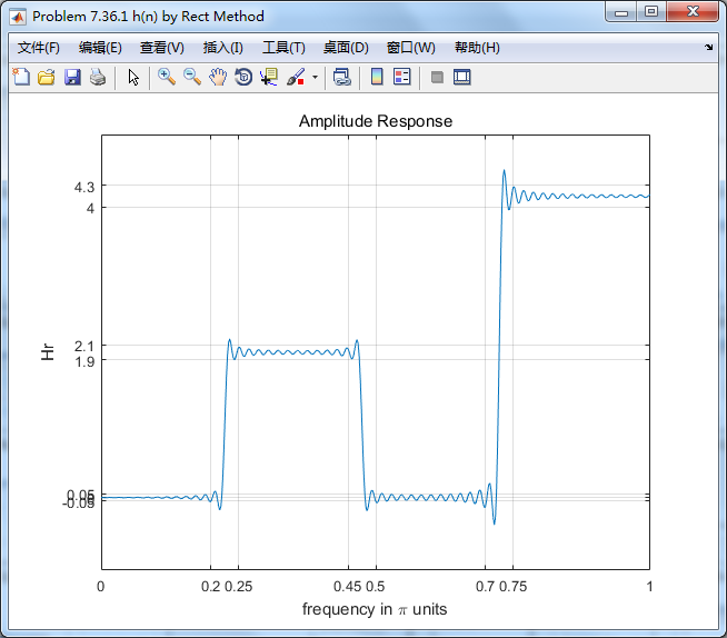
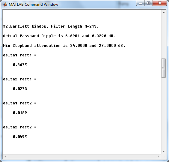
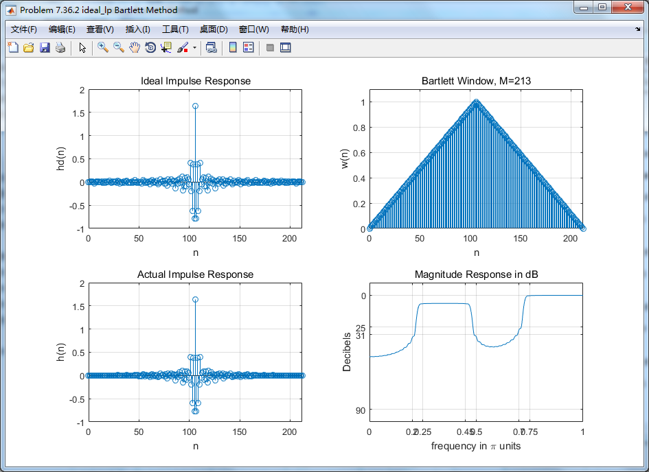
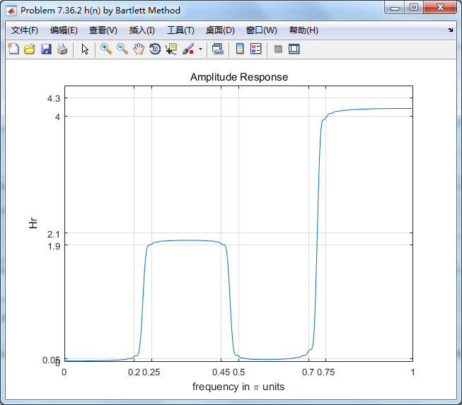
窗函数法,使用了矩形窗、三角窗、Hann窗、Hamming窗、Blackman窗、Kaiser窗,
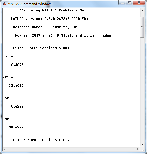
1、Rectangular窗

2、Bartlett三角窗
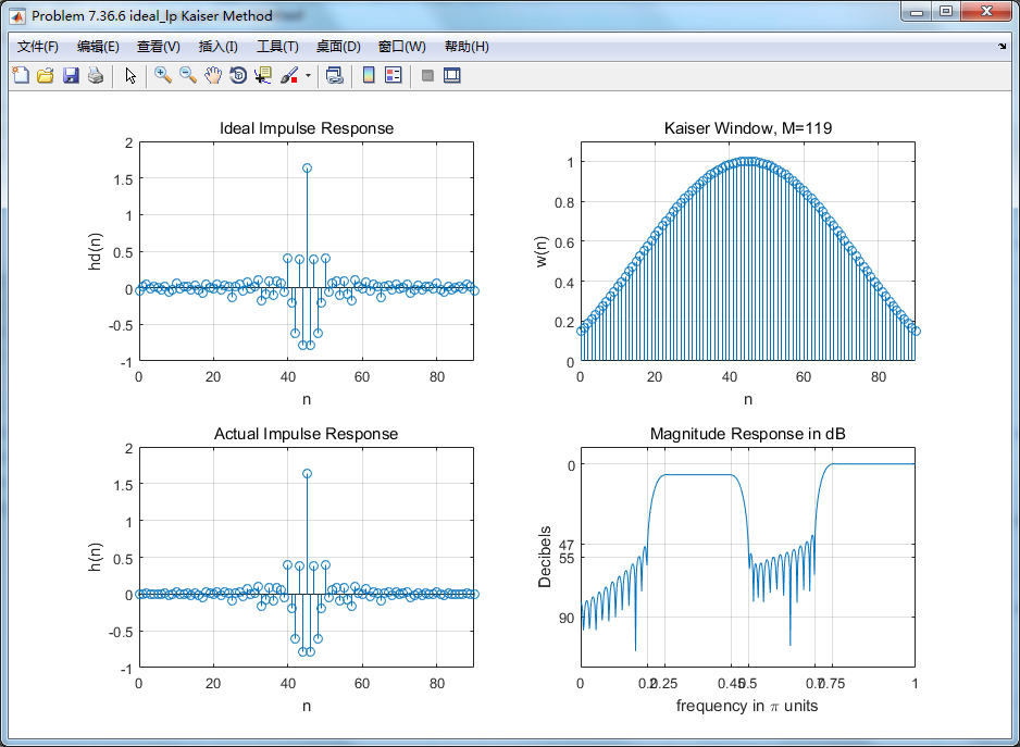
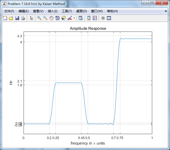
3、Hann、Hamming窗、Blackman窗的图这里不放了,直接放Kaiser窗的结果

4、频率采样方法


5、PM法
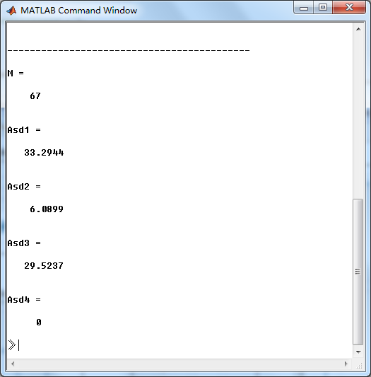
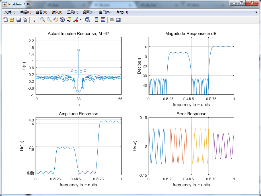

6、小结
以上用了窗函数法、频率采样法、Parks-McClellan法,下面对其得到的滤波器长度作对比,
| 序号 | 设 计 方 法 |
滤波器长度 M |
阻带衰减 As(dB) |
| 1 |
Rectangular矩形窗 |
227 | 28 |
| 2 | Bartlett三角窗 | 213 | 27 |
| 3 | Hann窗 | 125 | 41 |
| 4 | Hamming窗 | 133 | 49 |
| 5 | Blackman窗 | 221 | 68 |
| 6 | Kaiser窗 | 91 | 39 |
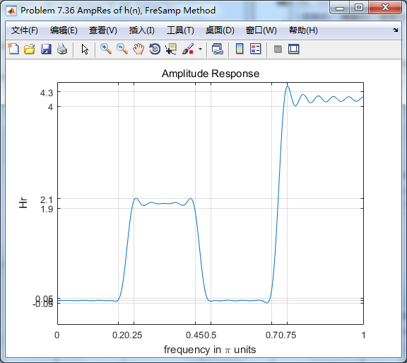
| 7 | 频率采样法 | 81 | 47 |
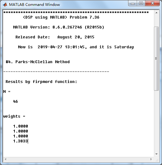
| 8 | Parks-McClellan法 | 67 | 30 |
结合滤波器指标要求和实际情况,Kaiser窗、频率采样法和P-M法可以采用。
《DSP using MATLAB》Problem 7.36的更多相关文章
- 《DSP using MATLAB》Problem 5.36
第1小题 代码: %% ++++++++++++++++++++++++++++++++++++++++++++++++++++++++++++++++++++++++++++++++++++++++ ...
- 《DSP using MATLAB》Problem 8.36
上代码: function [wpLP, wsLP, alpha] = lp2lpfre(wplp, wslp) % Band-edge frequency conversion from lowpa ...
- 《DSP using MATLAB》Problem 4.15
只会做前两个, 代码: %% ---------------------------------------------------------------------------- %% Outpu ...
- 《DSP using MATLAB》Problem 7.27
代码: %% ++++++++++++++++++++++++++++++++++++++++++++++++++++++++++++++++++++++++++++++++ %% Output In ...
- 《DSP using MATLAB》Problem 7.26
注意:高通的线性相位FIR滤波器,不能是第2类,所以其长度必须为奇数.这里取M=31,过渡带里采样值抄书上的. 代码: %% +++++++++++++++++++++++++++++++++++++ ...
- 《DSP using MATLAB》Problem 7.25
代码: %% ++++++++++++++++++++++++++++++++++++++++++++++++++++++++++++++++++++++++++++++++ %% Output In ...
- 《DSP using MATLAB》Problem 7.24
又到清明时节,…… 注意:带阻滤波器不能用第2类线性相位滤波器实现,我们采用第1类,长度为基数,选M=61 代码: %% +++++++++++++++++++++++++++++++++++++++ ...
- 《DSP using MATLAB》Problem 7.23
%% ++++++++++++++++++++++++++++++++++++++++++++++++++++++++++++++++++++++++++++++++ %% Output Info a ...
- 《DSP using MATLAB》Problem 7.16
使用一种固定窗函数法设计带通滤波器. 代码: %% ++++++++++++++++++++++++++++++++++++++++++++++++++++++++++++++++++++++++++ ...
随机推荐
- MVC 传递数据 从前台到后台,包括单个对象,多个对象,集合
MVC 传递数据 从前台到后台,包括单个对象,多个对象,集合 1.基本数据类型 我们常见有传递 int, string, bool, double, decimal 等类型. 需要注意的是前台传递的参 ...
- Java 局部变量
Java 局部变量 局部变量声明在方法.构造方法或者语句块中: 局部变量在方法.构造方法.或者语句块被执行的时候创建,当它们执行完成后,变量将会被销毁: 访问修饰符不能用于局部变量: 局部变量只在声明 ...
- jmeter遇到的问题:java.net.ConnectException: Connection refused: connect
1.使用jmeter执行脚本,在察看结果树的的响应数据中看到的错误提示如下: java.net.ConnectException: Connection refused: connect at jav ...
- Java 基础 - 装箱, 拆箱
总结 1-装箱过程是通过调用包装器的valueOf方法实现的,而拆箱过程是通过调用包装器的 xxxValue方法实现的.(xxx代表对应的基本数据类型).例如:在装箱的时候自动调用的是Integer的 ...
- .net下MVC中使用Tuple分页查询数据
主要是在DAL层写查询分页的代码. 例如DAL层上代码: public Tuple<List<WxBindDto>, int> GetMbersInfo(int start, ...
- 那些年,我们见过的 Java 服务端“问题”
导读 明代著名的心学集大成者王阳明先生在<传习录>中有云: 道无精粗,人之所见有精粗.如这一间房,人初进来,只见一个大规模如此.处久,便柱壁之类,一一看得明白.再久,如柱上有些文藻,细细都 ...
- day33 序列类型,绑定方法,类方法,静态方法,封装继承和多态
Python之路,Day20 = 序列类型,绑定方法,类方法,静态方法,封装继承和多态 序列是指有序的队列,重点在"有序". 一.Python中序列的分类 Python中的序列主要 ...
- (转)HttpURLConnection中设置网络超时
转:http://www.xd-tech.com.cn/blog/article.asp?id=37 Java中可以使用HttpURLConnection来请求WEB资源.HttpURLConnect ...
- STM32F4X 关于MDK上虚拟串口调试
1. 下载安装VSPD 自行百度安装后,利用VSPD将PC上的两个虚拟串口连接起来.如图我将COM1 和COM2连接起来. a. 点击Addr pair. 可以看到Virtual ports上将两个虚 ...
- Mysql优化系列之查询性能优化前篇3(必须知道的几个事实)
事实一:临时表没有任何索引 最常见的临时表莫过于在from子句中写子查询,遇到这种情况,Mysql会先将其查询结果放到一张临时表中, 然后将这个临时表当做普通表对待 事实二:执行计划优化 大多数的sq ...