《DSP using MATLAB》Problem 7.33

代码：

%% ++++++++++++++++++++++++++++++++++++++++++++++++++++++++++++++++++++++++++++++++
%%            Output Info about this m-file
fprintf('\n***********************************************************\n');
fprintf('        <DSP using MATLAB> Problem 7.33 \n\n');

banner();
%% ++++++++++++++++++++++++++++++++++++++++++++++++++++++++++++++++++++++++++++++++

ws1 = 0.44*pi; wp1 = 0.49*pi; wp2 = 0.51*pi; ws2=0.56*pi; As = 30; Rp = 1.0;
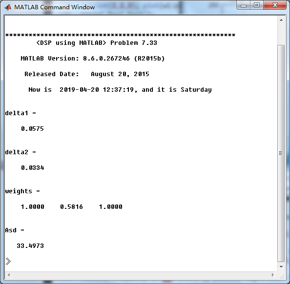
[delta1, delta2] = db2delta(Rp, As)

weights = [1  delta2/delta1  1]
deltaH = max([delta1,delta2]); deltaL = min([delta1,delta2]);

%Dw = min((wp1-ws1), (ws2-wp2));
%M = ceil((-20*log10((delta1*delta2)^(1/2)) - 13) / (2.285*Dw) + 1)

M = 51;
f = [ 0  ws1 wp1 wp2 ws2  pi]/pi;
m = [ 0   0  1   1   0  0];

h = firpm(M-1, f, m, weights);
[db, mag, pha, grd, w] = freqz_m(h, [1]);
delta_w = 2*pi/1000;
ws1i = floor(ws1/delta_w)+1; wp1i = floor(wp1/delta_w)+1;
wp2i = floor(wp2/delta_w)+1; ws2i = floor(ws2/delta_w)+1;

Asd = -max(db(1:ws1i))

%[Hr, ww, a, L] = Hr_Type1(h);
[Hr,omega,P,L] = ampl_res(h);
l = 0:M-1;

%% -------------------------------------------------
%%                    Plot
%% -------------------------------------------------  

figure('NumberTitle', 'off', 'Name', 'Problem 7.33 Parks-McClellan Method')
set(gcf,'Color','white'); 

subplot(2,2,1); stem(l, h); axis([-1, M, -0.1, 0.1]); grid on;
xlabel('n'); ylabel('h(n)'); title('Actual Impulse Response, M=51');
set(gca,'XTickMode','manual','XTick',[0,M-1])
set(gca,'YTickMode','manual','YTick',[-0.3:0.1:0.4])

subplot(2,2,2); plot(w/pi, db); axis([0, 1, -80, 10]); grid on;
xlabel('frequency in \pi units'); ylabel('Decibels'); title('Magnitude Response in dB ');
set(gca,'XTickMode','manual','XTick',f)
set(gca,'YTickMode','manual','YTick',[-60,-30,0]);
set(gca,'YTickLabelMode','manual','YTickLabel',['60';'30';' 0']);

subplot(2,2,3); plot(omega/pi, Hr); axis([0, 1, -0.2, 1.2]); grid on;
xlabel('frequency in \pi nuits'); ylabel('Hr(w)'); title('Amplitude Response');
set(gca,'XTickMode','manual','XTick',f)
set(gca,'YTickMode','manual','YTick',[0,1]);

delta_w = 2*pi/1000; 

subplot(2,2,4); axis([0, 1, -deltaH, deltaH]);
sb1w = omega(1:1:ws1i)/pi; sb1e = (Hr(1:1:ws1i)-m(1)); %sb1e = (Hr(1:1:ws1i)-m(1))*weights(1);
pbw = omega(wp1i:wp2i)/pi; pbe = (Hr(wp1i:wp2i)-m(3)); %pbe = (Hr(wp1i:wp2i)-m(3))*weights(2);
sb2w = omega(ws2i:501)/pi; sb2e = (Hr(ws2i:501)-m(5)); %sb2e = (Hr(ws2i:501)-m(5))*weights(3);
plot(sb1w,sb1e,pbw,pbe,sb2w,sb2e); grid on;
xlabel('frequency in \pi units'); ylabel('Hr(w)'); title('Error Response'); %title('Weighted Error');
set(gca,'XTickMode','manual','XTick',f);
%set(gca,'YTickMode','manual','YTick',[-deltaH,0,deltaH]);

figure('NumberTitle', 'off', 'Name', 'Problem 7.33 AmpRes of h(n), Parks-McClellan Method')
set(gcf,'Color','white'); 

plot(omega/pi, Hr); grid on; %axis([0 1 -100 10]);
xlabel('frequency in \pi units'); ylabel('Hr'); title('Amplitude Response');
set(gca,'YTickMode','manual','YTick',[-0.0334,0, 0.0334,1,1.057]);
%set(gca,'YTickLabelMode','manual','YTickLabel',['90';'40';' 0']);
set(gca,'XTickMode','manual','XTick',[0,0.44,0.49,0.51,0.56,1]);

%% -------------------------------------------------------
%%       Input is given, and we want the Output
%% -------------------------------------------------------
num = 200; mean_val=0; variance=1;
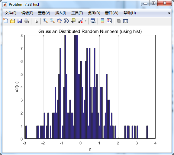
x2 = mean_val + sqrt(variance)*randn(num,1);
n_x2 = 0:num-1;
x_axis = min(x2):0.02:max(x2);

figure('NumberTitle', 'off', 'Name', 'Problem 7.33 hist');
set(gcf,'Color','white');
%hist(x1,x_axis);
hist(x2,100);
title('Gaussian Distributed Random Numbers (using hist)');
xlabel('n'); ylabel('x2(n)'); grid on;

figure('NumberTitle', 'off', 'Name', 'Problem 7.33 bar');
set(gcf,'Color','white');
%[counts,binlocal] = hist(x1, x_axis);
[counts,binlocal] = hist(x2, 100);
counts = counts/num;
bar(binlocal, counts, 1); title('Gaussian Distributed Random Numbers (using bar)');
xlabel('n'); ylabel('x2(n)'); grid on;

% Input
n_x3 = [0:1:num-1];
x3 = 2*cos(n_x3*pi/2);
[x,n_x] = sigadd (x2, n_x2, x3, n_x3);

y = filter(h, 1, x);
n_y = n_x;

figure('NumberTitle', 'off', 'Name', 'Problem 7.33 Input[x(n)] and Output[y(n)]');
set(gcf,'Color','white');
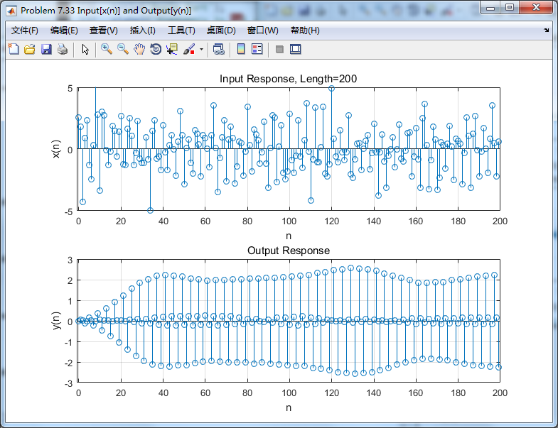
subplot(2,1,1); stem(n_x, x); axis([-1, 200, -5, 5]); grid on;
xlabel('n'); ylabel('x(n)'); title('Input Response, Length=200');
subplot(2,1,2); stem(n_y, y); axis([-1, 200, -3, 3]); grid on;
xlabel('n'); ylabel('y(n)'); title('Output Response');

% ---------------------------
%    DTFT of x and y
% ---------------------------
MM = 500;
[X, w1] = dtft1(x, n_x, MM);
[Y, w1] = dtft1(y, n_y, MM);

magX = abs(X); angX = angle(X); realX = real(X); imagX = imag(X);
magY = abs(Y); angY = angle(Y); realY = real(Y); imagY = imag(Y);

figure('NumberTitle', 'off', 'Name', 'Problem 7.33 DTFT of Input[x(n)]')
set(gcf,'Color','white');
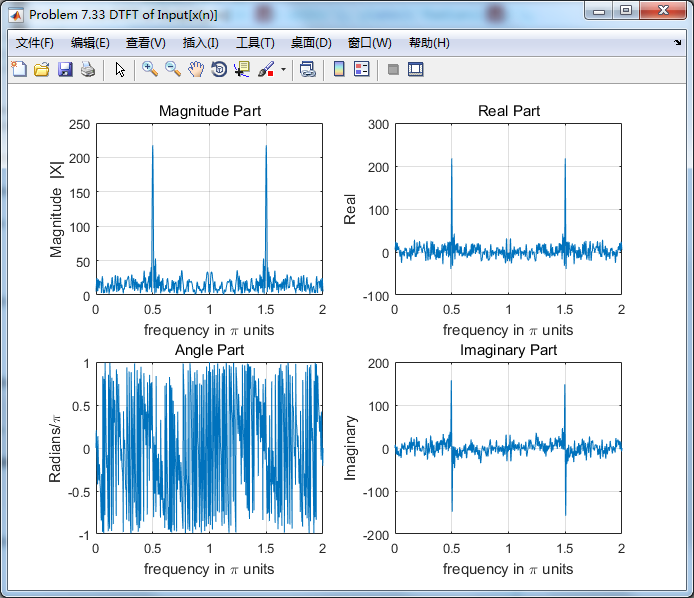
subplot(2,2,1); plot(w1/pi,magX); grid on; %axis([0,2,0,15]);
title('Magnitude Part');
xlabel('frequency in \pi units'); ylabel('Magnitude  |X|');
subplot(2,2,3); plot(w1/pi, angX/pi); grid on; axis([0,2,-1,1]);
title('Angle Part');
xlabel('frequency in \pi units'); ylabel('Radians/\pi');

subplot(2,2,2); plot(w1/pi, realX); grid on;
title('Real Part');
xlabel('frequency in \pi units'); ylabel('Real');
subplot(2,2,4); plot(w1/pi, imagX); grid on;
title('Imaginary Part');
xlabel('frequency in \pi units'); ylabel('Imaginary');

figure('NumberTitle', 'off', 'Name', 'Problem 7.33 DTFT of Output[y(n)]')
set(gcf,'Color','white');
subplot(2,2,1); plot(w1/pi,magY); grid on; %axis([0,2,0,15]);
title('Magnitude Part');
xlabel('frequency in \pi units'); ylabel('Magnitude  |Y|');
subplot(2,2,3); plot(w1/pi, angY/pi); grid on; axis([0,2,-1,1]);
title('Angle Part');
xlabel('frequency in \pi units'); ylabel('Radians/\pi');

subplot(2,2,2); plot(w1/pi, realY); grid on;
title('Real Part');
xlabel('frequency in \pi units'); ylabel('Real');
subplot(2,2,4); plot(w1/pi, imagY); grid on;
title('Imaginary Part');
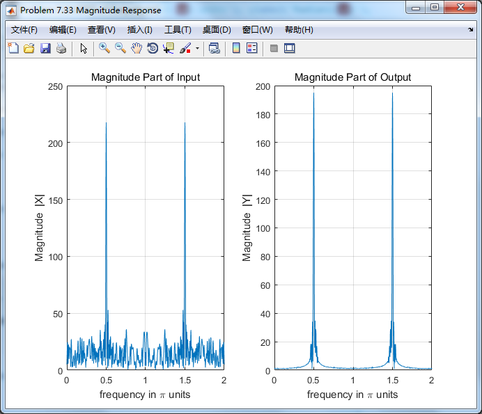
xlabel('frequency in \pi units'); ylabel('Imaginary');

figure('NumberTitle', 'off', 'Name', 'Problem 7.33 Magnitude Response')
set(gcf,'Color','white');
subplot(1,2,1); plot(w1/pi,magX); grid on; %axis([0,2,0,15]);
title('Magnitude Part of Input');
xlabel('frequency in \pi units'); ylabel('Magnitude  |X|');
subplot(1,2,2); plot(w1/pi,magY); grid on; %axis([0,2,0,15]);
title('Magnitude Part of Output');
xlabel('frequency in \pi units'); ylabel('Magnitude  |Y|');

　　运行结果：

设计一个50阶（即长度M=51）的线性相位FIR，通带宽度不超过0.02π，阻带衰减达到30dB，

最后要把输入中的高斯噪声过滤掉。

As=33dB，满足设计要求。

用P-M方法设计的脉冲响应幅度谱，

振幅谱

输入信号

滤波前后，输入数出对比

输入输出的谱：

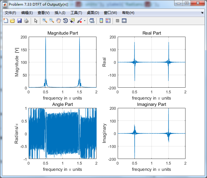
右下图可见，随即噪声分量已滤除，仅留0.5π频率分量，效果良好。