吴裕雄--天生自然 python数据分析：医疗费数据分析

import numpy as np
import pandas as pd
import os
import matplotlib.pyplot as pl
import seaborn as sns
import warnings
warnings.filterwarnings('ignore')
data = pd.read_csv('F:\\kaggleDataSet\\MedicalCostPersonal\\insurance.csv')

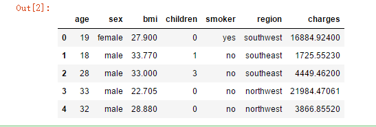
data.head()

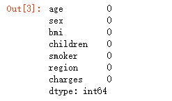
data.isnull().sum()

from sklearn.preprocessing import LabelEncoder
#sex
le = LabelEncoder()
le.fit(data.sex.drop_duplicates())
data.sex = le.transform(data.sex)
# smoker or not
le.fit(data.smoker.drop_duplicates())
data.smoker = le.transform(data.smoker)
#region
le.fit(data.region.drop_duplicates())
data.region = le.transform(data.region)

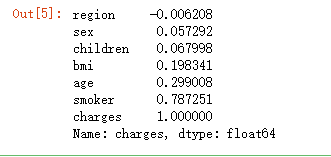
data.corr()['charges'].sort_values()

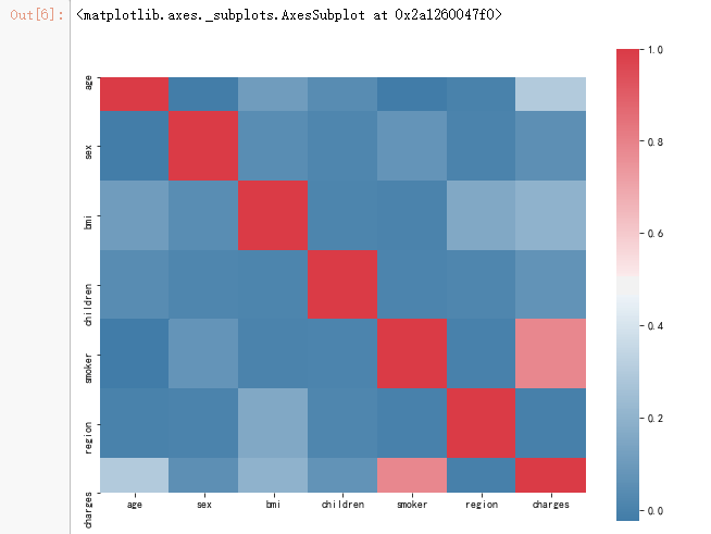
f, ax = pl.subplots(figsize=(10, 8))
corr = data.corr()
sns.heatmap(corr, mask=np.zeros_like(corr, dtype=np.bool), cmap=sns.diverging_palette(240,10,as_cmap=True),square=True, ax=ax)

from bokeh.io import output_notebook, show
from bokeh.plotting import figure
output_notebook()
import scipy.special
from bokeh.layouts import gridplot
from bokeh.plotting import figure, show, output_file
p = figure(title="Distribution of charges",tools="save",background_fill_color="#E8DDCB")
hist, edges = np.histogram(data.charges)
p.quad(top=hist, bottom=0, left=edges[:-1], right=edges[1:],fill_color="#036564", line_color="#033649")
p.xaxis.axis_label = 'x'
p.yaxis.axis_label = 'Pr(x)'
show(gridplot(p,ncols = 2, plot_width=400, plot_height=400, toolbar_location=None))

f= pl.figure(figsize=(12,5))

ax=f.add_subplot(121)
sns.distplot(data[(data.smoker == 1)]["charges"],color='c',ax=ax)
ax.set_title('Distribution of charges for smokers')

ax=f.add_subplot(122)
sns.distplot(data[(data.smoker == 0)]['charges'],color='b',ax=ax)
ax.set_title('Distribution of charges for non-smokers')

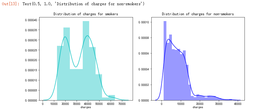
sns.catplot(x="smoker", kind="count",hue = 'sex', palette="pink", data=data)

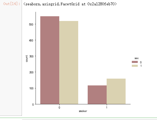
sns.catplot(x="sex", y="charges", hue="smoker",kind="violin", data=data, palette = 'magma')

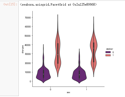
pl.figure(figsize=(12,5))
pl.title("Box plot for charges of women")
sns.boxplot(y="smoker", x="charges", data =  data[(data.sex == 1)] , orient="h", palette = 'magma')

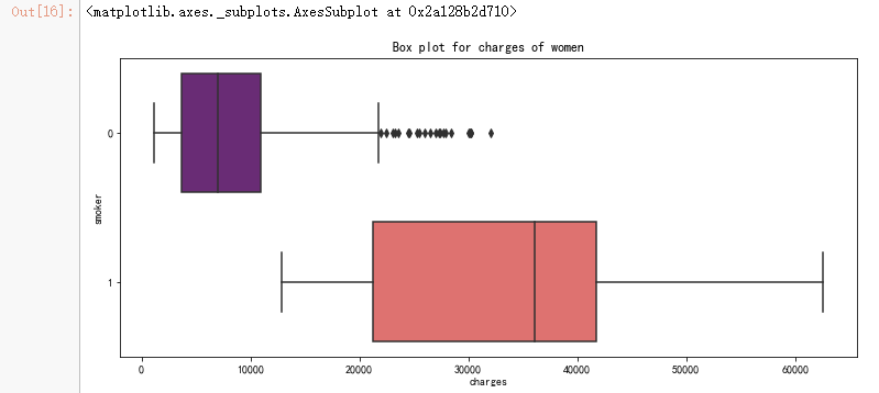
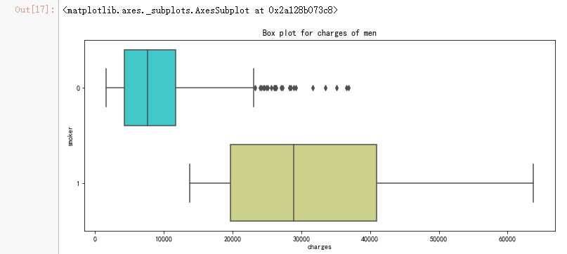
pl.figure(figsize=(12,5))
pl.title("Box plot for charges of men")
sns.boxplot(y="smoker", x="charges", data =  data[(data.sex == 0)] , orient="h", palette = 'rainbow')

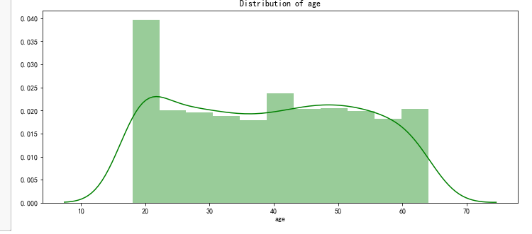
pl.figure(figsize=(12,5))
pl.title("Distribution of age")
ax = sns.distplot(data["age"], color = 'g')

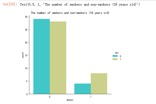
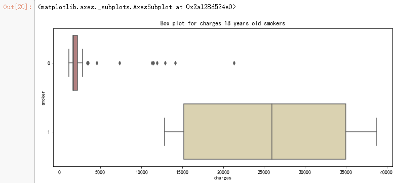
sns.catplot(x="smoker", kind="count",hue = 'sex', palette="rainbow", data=data[(data.age == 18)])
pl.title("The number of smokers and non-smokers (18 years old)")

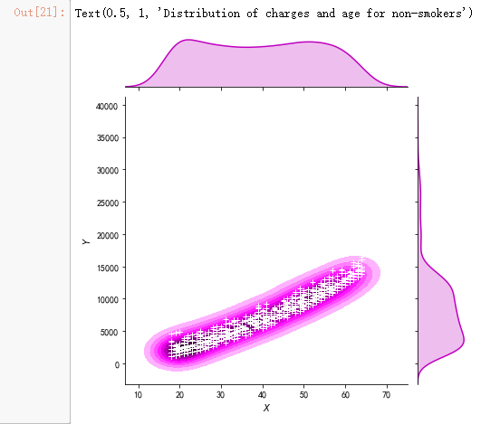
g = sns.jointplot(x="age", y="charges", data = data[(data.smoker == 0)],kind="kde", color="m")
g.plot_joint(pl.scatter, c="w", s=30, linewidth=1, marker="+")
g.ax_joint.collections[0].set_alpha(0)
g.set_axis_labels("$X$", "$Y$")
ax.set_title('Distribution of charges and age for non-smokers')

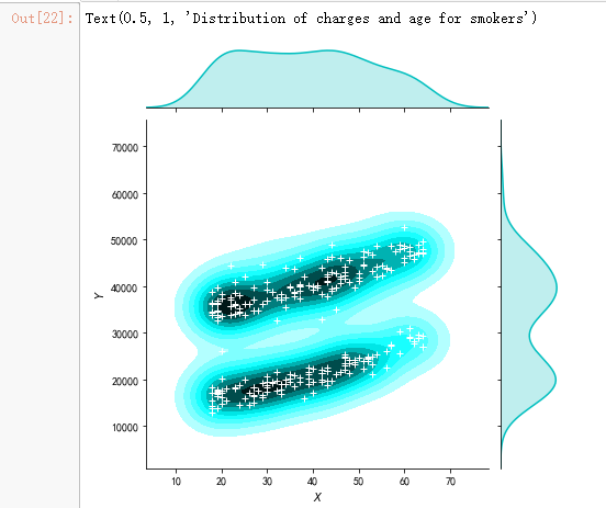
g = sns.jointplot(x="age", y="charges", data = data[(data.smoker == 1)],kind="kde", color="c")
g.plot_joint(pl.scatter, c="w", s=30, linewidth=1, marker="+")
g.ax_joint.collections[0].set_alpha(0)
g.set_axis_labels("$X$", "$Y$")
ax.set_title('Distribution of charges and age for smokers')

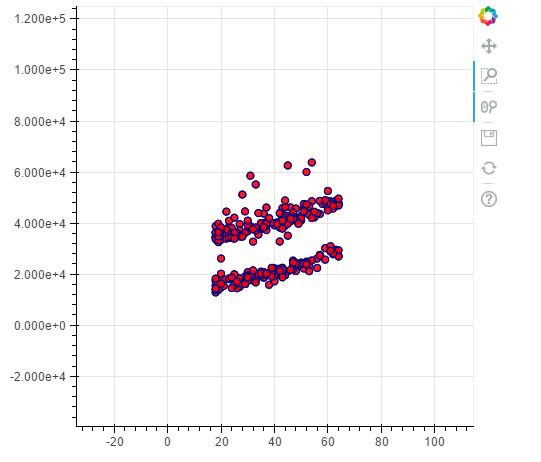
#non - smokers
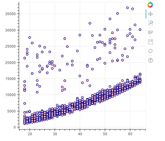
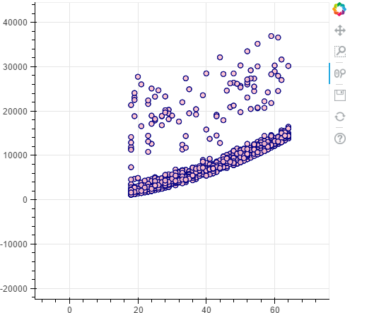
p = figure(plot_width=500, plot_height=450)
p.circle(x=data[(data.smoker == 0)].age,y=data[(data.smoker == 0)].charges, size=7, line_color="navy", fill_color="pink", fill_alpha=0.9)

show(p)

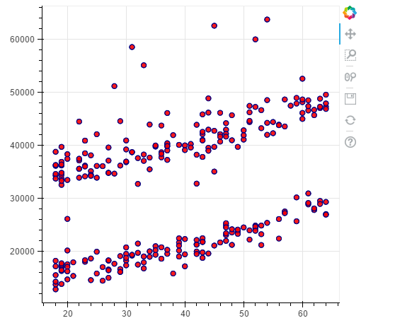
#smokers
p = figure(plot_width=500, plot_height=450)
p.circle(x=data[(data.smoker == 1)].age,y=data[(data.smoker == 1)].charges, size=7, line_color="navy", fill_color="red", fill_alpha=0.9)
show(p)

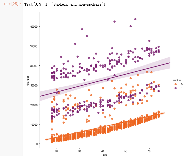
sns.lmplot(x="age", y="charges", hue="smoker", data=data, palette = 'inferno_r', size = 7)
ax.set_title('Smokers and non-smokers')

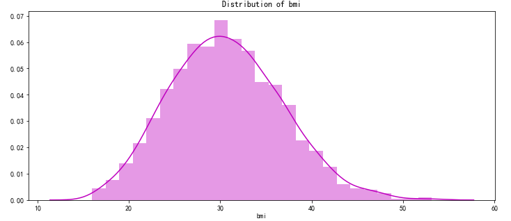
pl.figure(figsize=(12,5))
pl.title("Distribution of bmi")
ax = sns.distplot(data["bmi"], color = 'm')

pl.figure(figsize=(12,5))
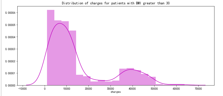
pl.title("Distribution of charges for patients with BMI greater than 30")
ax = sns.distplot(data[(data.bmi >= 30)]['charges'], color = 'm')

pl.figure(figsize=(12,5))
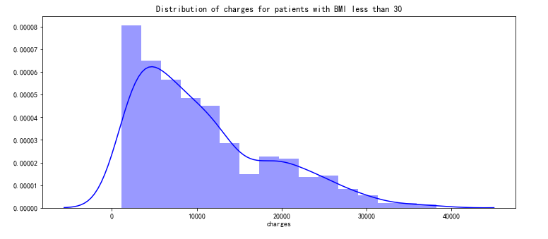
pl.title("Distribution of charges for patients with BMI less than 30")
ax = sns.distplot(data[(data.bmi < 30)]['charges'], color = 'b')

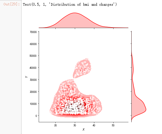
g = sns.jointplot(x="bmi", y="charges", data = data,kind="kde", color="r")
g.plot_joint(pl.scatter, c="w", s=30, linewidth=1, marker="+")
g.ax_joint.collections[0].set_alpha(0)
g.set_axis_labels("$X$", "$Y$")
ax.set_title('Distribution of bmi and charges')

pl.figure(figsize=(10,6))
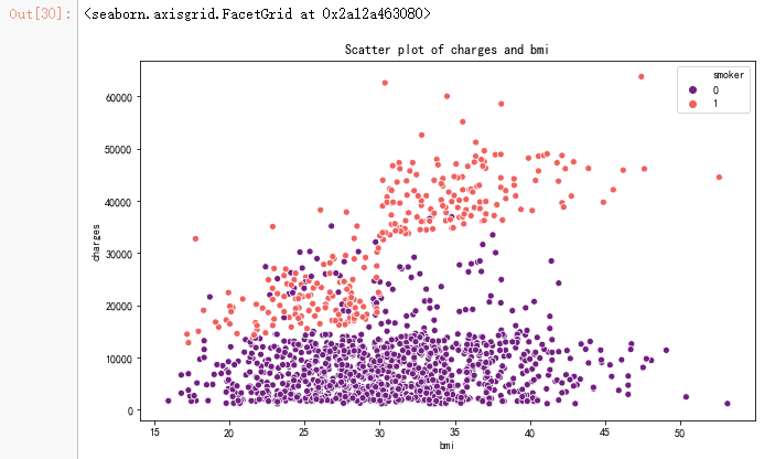
ax = sns.scatterplot(x='bmi',y='charges',data=data,palette='magma',hue='smoker')
ax.set_title('Scatter plot of charges and bmi')

sns.lmplot(x="bmi", y="charges", hue="smoker", data=data, palette = 'magma', size = 8)

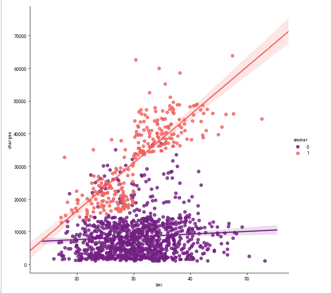
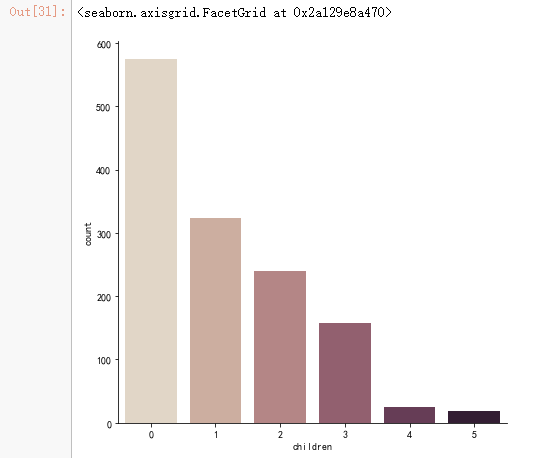
sns.catplot(x="children", kind="count", palette="ch:.25", data=data, size = 6)

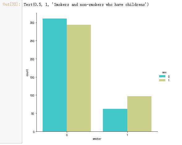
sns.catplot(x="smoker", kind="count", palette="rainbow",hue = "sex",
            data=data[(data.children > 0)], size = 6)
ax.set_title('Smokers and non-smokers who have childrens')

from sklearn.linear_model import LinearRegression
from sklearn.model_selection import train_test_split
from sklearn.preprocessing import PolynomialFeatures
from sklearn.metrics import r2_score,mean_squared_error
from sklearn.ensemble import RandomForestRegressor

x = data.drop(['charges'], axis = 1)
y = data.charges

x_train,x_test,y_train,y_test = train_test_split(x,y, random_state = 0)
lr = LinearRegression().fit(x_train,y_train)

y_train_pred = lr.predict(x_train)
y_test_pred = lr.predict(x_test)

print(lr.score(x_test,y_test))

X = data.drop(['charges','region'], axis = 1)
Y = data.charges

quad = PolynomialFeatures (degree = 2)
x_quad = quad.fit_transform(X)

X_train,X_test,Y_train,Y_test = train_test_split(x_quad,Y, random_state = 0)

plr = LinearRegression().fit(X_train,Y_train)

Y_train_pred = plr.predict(X_train)
Y_test_pred = plr.predict(X_test)

print(plr.score(X_test,Y_test))

forest = RandomForestRegressor(n_estimators = 100,criterion = 'mse',random_state = 1,n_jobs = -1)
forest.fit(x_train,y_train)
forest_train_pred = forest.predict(x_train)
forest_test_pred = forest.predict(x_test)

print('MSE train data: %.3f, MSE test data: %.3f' % (
mean_squared_error(y_train,forest_train_pred),
mean_squared_error(y_test,forest_test_pred)))
print('R2 train data: %.3f, R2 test data: %.3f' % (
r2_score(y_train,forest_train_pred),
r2_score(y_test,forest_test_pred)))

pl.figure(figsize=(10,6))

pl.scatter(forest_train_pred,forest_train_pred - y_train,c = 'black', marker = 'o', s = 35, alpha = 0.5,label = 'Train data')
pl.scatter(forest_test_pred,forest_test_pred - y_test,c = 'c', marker = 'o', s = 35, alpha = 0.7,label = 'Test data')
pl.xlabel('Predicted values')
pl.ylabel('Tailings')
pl.legend(loc = 'upper left')
pl.hlines(y = 0, xmin = 0, xmax = 60000, lw = 2, color = 'red')
pl.show()