吴裕雄--天生自然 PYTHON数据分析：基于Keras的CNN分析太空深处寻找系外行星数据

#We import libraries for linear algebra, graphs, and evaluation of results
import numpy as np
import matplotlib.pyplot as plt
from sklearn.linear_model import LinearRegression
from sklearn.preprocessing import StandardScaler
from sklearn.metrics import roc_curve, roc_auc_score
from scipy.ndimage.filters import uniform_filter1d

#Keras is a high level neural networks library, based on either tensorflow or theano
from keras.models import Sequential, Model
from keras.layers import Conv1D, MaxPool1D, Dense, Dropout, Flatten, BatchNormalization, Input, concatenate, Activation
from keras.optimizers import Adam

INPUT_LIB = 'F:\\kaggleDataSet\\kepler-labelled\\'
raw_data = np.loadtxt(INPUT_LIB + 'exoTrain.csv', skiprows=1, delimiter=',')
x_train = raw_data[:, 1:]
y_train = raw_data[:, 0, np.newaxis] - 1.
raw_data = np.loadtxt(INPUT_LIB + 'exoTest.csv', skiprows=1, delimiter=',')
x_test = raw_data[:, 1:]
y_test = raw_data[:, 0, np.newaxis] - 1.
del raw_data

x_train = ((x_train - np.mean(x_train, axis=1).reshape(-1,1))/ np.std(x_train, axis=1).reshape(-1,1))
x_test = ((x_test - np.mean(x_test, axis=1).reshape(-1,1)) / np.std(x_test, axis=1).reshape(-1,1))

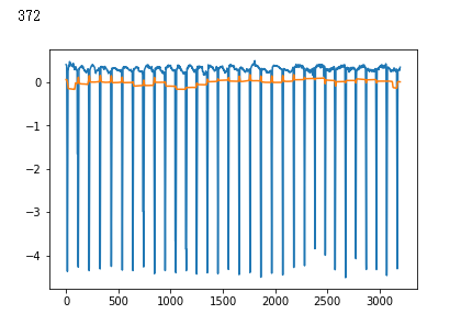
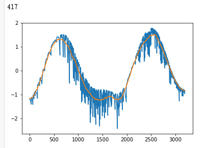
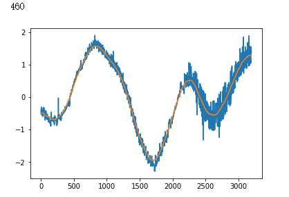
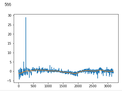
x_train = np.stack([x_train, uniform_filter1d(x_train, axis=1, size=200)], axis=2)
x_test = np.stack([x_test, uniform_filter1d(x_test, axis=1, size=200)], axis=2)

model = Sequential()
model.add(Conv1D(filters=8, kernel_size=11, activation='relu', input_shape=x_train.shape[1:]))
model.add(MaxPool1D(strides=4))
model.add(BatchNormalization())
model.add(Conv1D(filters=16, kernel_size=11, activation='relu'))
model.add(MaxPool1D(strides=4))
model.add(BatchNormalization())
model.add(Conv1D(filters=32, kernel_size=11, activation='relu'))
model.add(MaxPool1D(strides=4))
model.add(BatchNormalization())
model.add(Conv1D(filters=64, kernel_size=11, activation='relu'))
model.add(MaxPool1D(strides=4))
model.add(Flatten())
model.add(Dropout(0.5))
model.add(Dense(64, activation='relu'))
model.add(Dropout(0.25))
model.add(Dense(64, activation='relu'))
model.add(Dense(1, activation='sigmoid'))

def batch_generator(x_train, y_train, batch_size=32):
    """
    Gives equal number of positive and negative samples, and rotates them randomly in time
    """
    half_batch = batch_size // 2
    x_batch = np.empty((batch_size, x_train.shape[1], x_train.shape[2]), dtype='float32')
    y_batch = np.empty((batch_size, y_train.shape[1]), dtype='float32')

    yes_idx = np.where(y_train[:,0] == 1.)[0]
    non_idx = np.where(y_train[:,0] == 0.)[0]

    while True:
        np.random.shuffle(yes_idx)
        np.random.shuffle(non_idx)

        x_batch[:half_batch] = x_train[yes_idx[:half_batch]]
        x_batch[half_batch:] = x_train[non_idx[half_batch:batch_size]]
        y_batch[:half_batch] = y_train[yes_idx[:half_batch]]
        y_batch[half_batch:] = y_train[non_idx[half_batch:batch_size]]

        for i in range(batch_size):
            sz = np.random.randint(x_batch.shape[1])
            x_batch[i] = np.roll(x_batch[i], sz, axis = 0)

        yield x_batch, y_batch

#Start with a slightly lower learning rate, to ensure convergence
model.compile(optimizer=Adam(1e-5), loss = 'binary_crossentropy', metrics=['accuracy'])
hist = model.fit_generator(batch_generator(x_train, y_train, 32),
                           validation_data=(x_test, y_test),
                           verbose=0, epochs=5,
                           steps_per_epoch=x_train.shape[1]//32)

#Then speed things up a little
model.compile(optimizer=Adam(4e-5), loss = 'binary_crossentropy', metrics=['accuracy'])
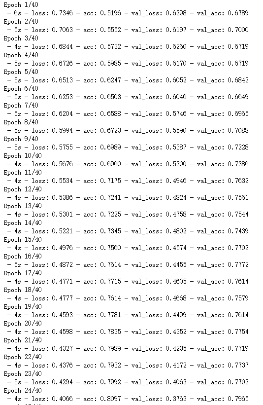
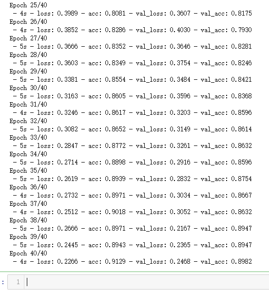
hist = model.fit_generator(batch_generator(x_train, y_train, 32),
                           validation_data=(x_test, y_test),
                           verbose=2, epochs=40,
                           steps_per_epoch=x_train.shape[1]//32)

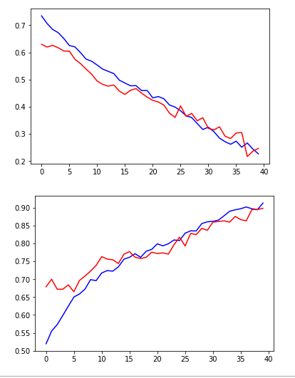
plt.plot(hist.history['loss'], color='b')
plt.plot(hist.history['val_loss'], color='r')
plt.show()
plt.plot(hist.history['acc'], color='b')
plt.plot(hist.history['val_acc'], color='r')
plt.show()

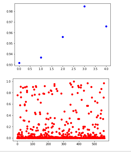
non_idx = np.where(y_test[:,0] == 0.)[0]
yes_idx = np.where(y_test[:,0] == 1.)[0]
y_hat = model.predict(x_test)[:,0]

plt.plot([y_hat[i] for i in yes_idx], 'bo')
plt.show()
plt.plot([y_hat[i] for i in non_idx], 'ro')
plt.show()

y_true = (y_test[:, 0] + 0.5).astype("int")
fpr, tpr, thresholds = roc_curve(y_true, y_hat)
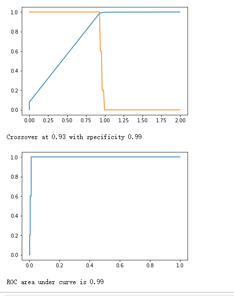
plt.plot(thresholds, 1.-fpr)
plt.plot(thresholds, tpr)
plt.show()
crossover_index = np.min(np.where(1.-fpr <= tpr))
crossover_cutoff = thresholds[crossover_index]
crossover_specificity = 1.-fpr[crossover_index]
print("Crossover at {0:.2f} with specificity {1:.2f}".format(crossover_cutoff, crossover_specificity))
plt.plot(fpr, tpr)
plt.show()
print("ROC area under curve is {0:.2f}".format(roc_auc_score(y_true, y_hat)))

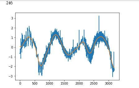
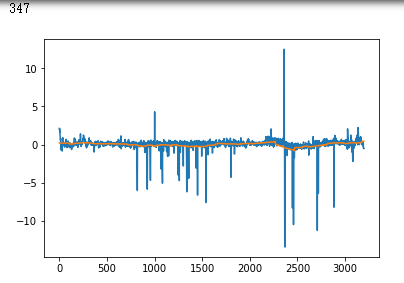
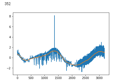
false_positives = np.where(y_hat * (1. - y_test) > 0.5)[0]
for i in non_idx:
    if y_hat[i] > crossover_cutoff:
        print(i)
        plt.plot(x_test[i])
        plt.show()