吴裕雄--天生自然 PYTHON数据分析：威斯康星乳腺癌(诊断)数据分析（续一）

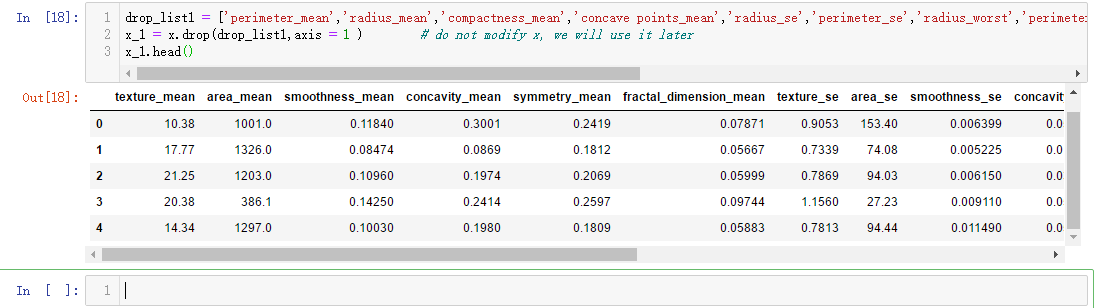
drop_list1 = ['perimeter_mean','radius_mean','compactness_mean','concave points_mean','radius_se','perimeter_se','radius_worst','perimeter_worst','compactness_worst','concave points_worst','compactness_se','concave points_se','texture_worst','area_worst']
x_1 = x.drop(drop_list1,axis = 1 )        # do not modify x, we will use it later
x_1.head()

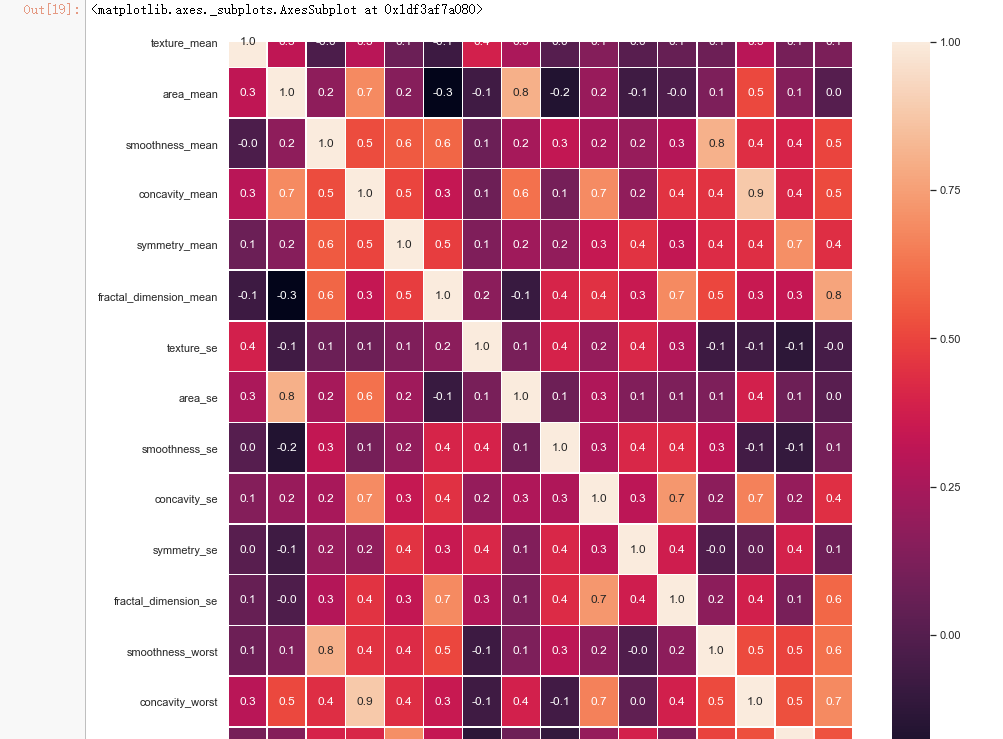
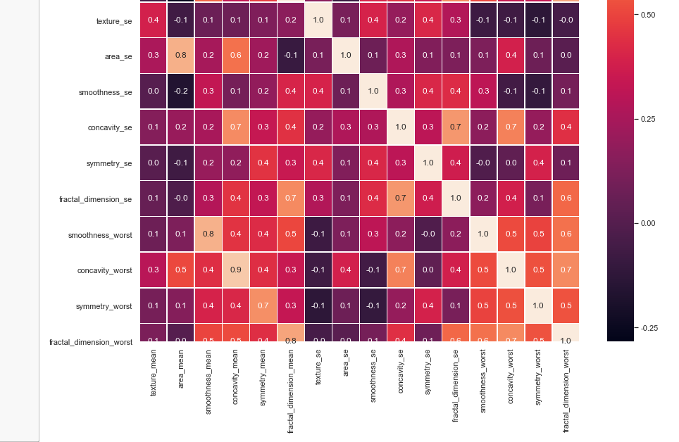
#correlation map
f,ax = plt.subplots(figsize=(14, 14))
sns.heatmap(x_1.corr(), annot=True, linewidths=.5, fmt= '.1f',ax=ax)

from sklearn.model_selection import train_test_split
from sklearn.ensemble import RandomForestClassifier
from sklearn.metrics import f1_score,confusion_matrix
from sklearn.metrics import accuracy_score

# split data train 70 % and test 30 %
x_train, x_test, y_train, y_test = train_test_split(x_1, y, test_size=0.3, random_state=42)

#random forest classifier with n_estimators=10 (default)
clf_rf = RandomForestClassifier(random_state=43)
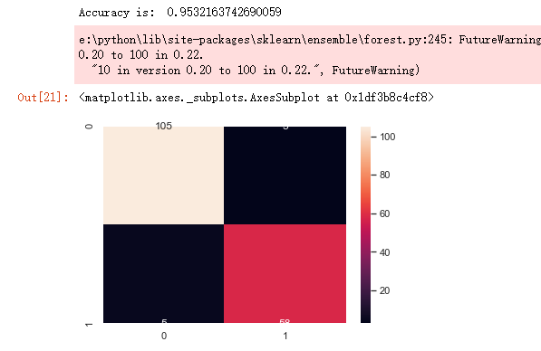
clr_rf = clf_rf.fit(x_train,y_train)

ac = accuracy_score(y_test,clf_rf.predict(x_test))
print('Accuracy is: ',ac)
cm = confusion_matrix(y_test,clf_rf.predict(x_test))
sns.heatmap(cm,annot=True,fmt="d")

from sklearn.feature_selection import SelectKBest
from sklearn.feature_selection import chi2
# find best scored 5 features
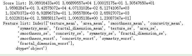
select_feature = SelectKBest(chi2, k=5).fit(x_train, y_train)

print('Score list:', select_feature.scores_)
print('Feature list:', x_train.columns)

x_train_2 = select_feature.transform(x_train)
x_test_2 = select_feature.transform(x_test)
#random forest classifier with n_estimators=10 (default)
clf_rf_2 = RandomForestClassifier()
clr_rf_2 = clf_rf_2.fit(x_train_2,y_train)
ac_2 = accuracy_score(y_test,clf_rf_2.predict(x_test_2))
print('Accuracy is: ',ac_2)
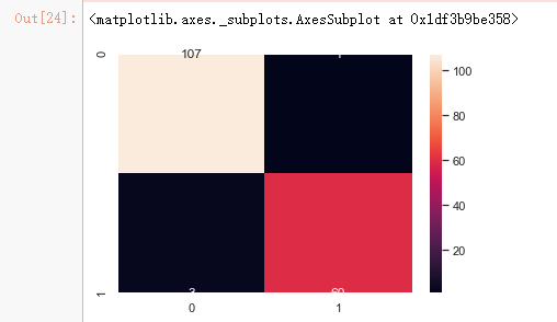
cm_2 = confusion_matrix(y_test,clf_rf_2.predict(x_test_2))
sns.heatmap(cm_2,annot=True,fmt="d")

from sklearn.feature_selection import RFE
# Create the RFE object and rank each pixel
clf_rf_3 = RandomForestClassifier()
rfe = RFE(estimator=clf_rf_3, n_features_to_select=5, step=1)
rfe = rfe.fit(x_train, y_train)

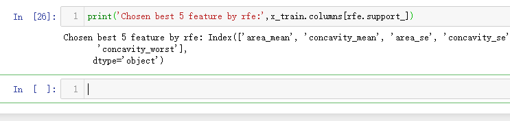
print('Chosen best 5 feature by rfe:',x_train.columns[rfe.support_])

from sklearn.feature_selection import RFECV

# The "accuracy" scoring is proportional to the number of correct classifications
clf_rf_4 = RandomForestClassifier()
rfecv = RFECV(estimator=clf_rf_4, step=1, cv=5,scoring='accuracy')   #5-fold cross-validation
rfecv = rfecv.fit(x_train, y_train)

print('Optimal number of features :', rfecv.n_features_)
print('Best features :', x_train.columns[rfecv.support_])

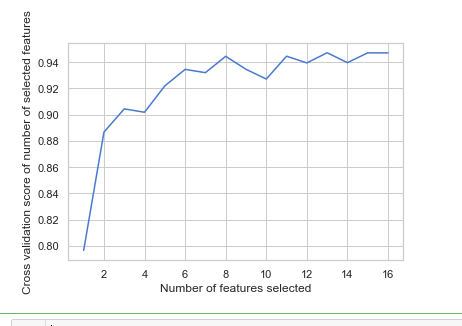
# Plot number of features VS. cross-validation scores
import matplotlib.pyplot as plt
plt.figure()
plt.xlabel("Number of features selected")
plt.ylabel("Cross validation score of number of selected features")
plt.plot(range(1, len(rfecv.grid_scores_) + 1), rfecv.grid_scores_)
plt.show()

clf_rf_5 = RandomForestClassifier()
clr_rf_5 = clf_rf_5.fit(x_train,y_train)
importances = clr_rf_5.feature_importances_
std = np.std([tree.feature_importances_ for tree in clf_rf.estimators_],
             axis=0)
indices = np.argsort(importances)[::-1]

# Print the feature ranking
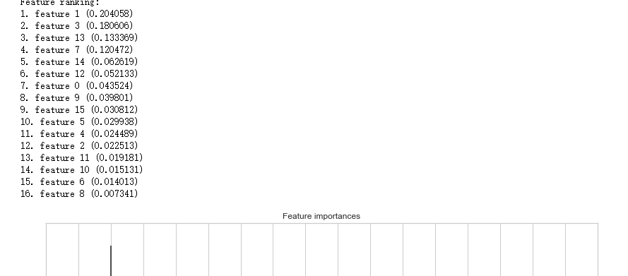
print("Feature ranking:")

for f in range(x_train.shape[1]):
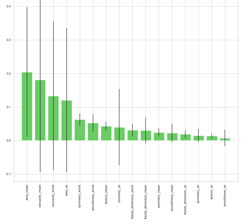
    print("%d. feature %d (%f)" % (f + 1, indices[f], importances[indices[f]]))

# Plot the feature importances of the forest

plt.figure(1, figsize=(14, 13))
plt.title("Feature importances")
plt.bar(range(x_train.shape[1]), importances[indices],
       color="g", yerr=std[indices], align="center")
plt.xticks(range(x_train.shape[1]), x_train.columns[indices],rotation=90)
plt.xlim([-1, x_train.shape[1]])
plt.show()

# split data train 70 % and test 30 %
x_train, x_test, y_train, y_test = train_test_split(x, y, test_size=0.3, random_state=42)
#normalization
x_train_N = (x_train-x_train.mean())/(x_train.max()-x_train.min())
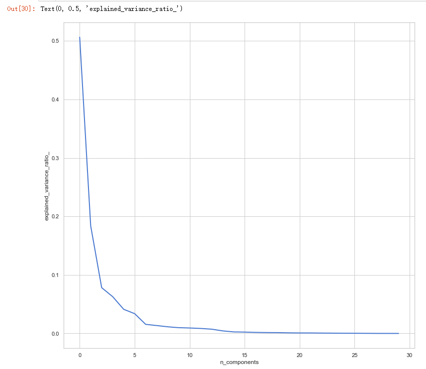
x_test_N = (x_test-x_test.mean())/(x_test.max()-x_test.min())

from sklearn.decomposition import PCA
pca = PCA()
pca.fit(x_train_N)

plt.figure(1, figsize=(14, 13))
plt.clf()
plt.axes([.2, .2, .7, .7])
plt.plot(pca.explained_variance_ratio_, linewidth=2)
plt.axis('tight')
plt.xlabel('n_components')
plt.ylabel('explained_variance_ratio_')