《DSP using MATLAB》Problem 8.41

代码：

%% ------------------------------------------------------------------------
%%            Output Info about this m-file
fprintf('\n***********************************************************\n');
fprintf('        <DSP using MATLAB> Problem 8.41.2 \n\n');

banner();
%% ------------------------------------------------------------------------

% Digital lowpass Filter Specifications:
wplp = 0.4*pi;                 % digital passband freq in rad
wslp = 0.5*pi;                 % digital stopband freq in rad
Rp = 1.0;                       % passband ripple in dB
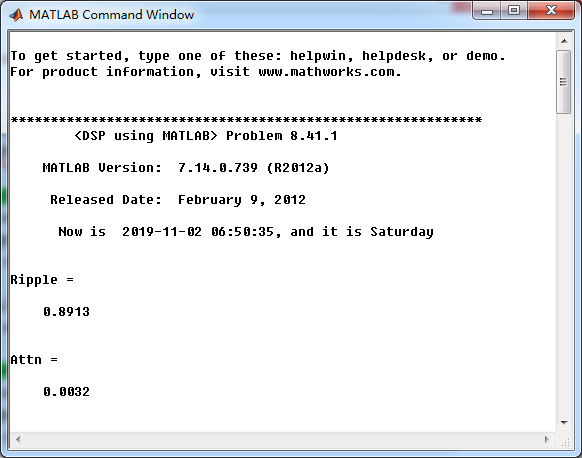
As = 50.0;                        % stopband attenuation in dB

Ripple = 10 ^ (-Rp/20)           % passband ripple in absolute
Attn = 10 ^ (-As/20)             % stopband attenuation in absolute

fprintf('\n*******Digital lowpass, Coefficients of DIRECT-form***********\n');
[blp, alp] = cheb2lpf(wplp, wslp, Rp, As);
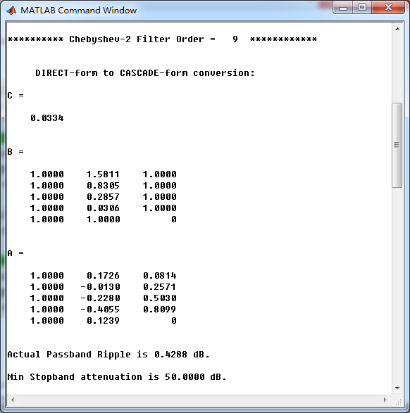
[C, B, A] = dir2cas(blp, alp)

% Calculation of Frequency Response:
[dblp, maglp, phalp, grdlp, wwlp] = freqz_m(blp, alp);

% ---------------------------------------------------------------
%    find Actual Passband Ripple and Min Stopband attenuation
% ---------------------------------------------------------------
delta_w = 2*pi/1000;
Rp_lp = -(min(dblp(1:1:ceil(wplp/delta_w)+1)));                            % Actual Passband Ripple

fprintf('\nActual Passband Ripple is %.4f dB.\n', Rp_lp);

As_lp = -round(max(dblp( ceil(wslp/delta_w)+1:1:501 )));                    % Min Stopband attenuation
fprintf('\nMin Stopband attenuation is %.4f dB.\n\n', As_lp);

%% -----------------------------------------------------------------
%%                             Plot
%% -----------------------------------------------------------------  

figure('NumberTitle', 'off', 'Name', 'Problem 8.41.1 Chebyshev-2 lowpass by cheb2lpf function')
set(gcf,'Color','white');
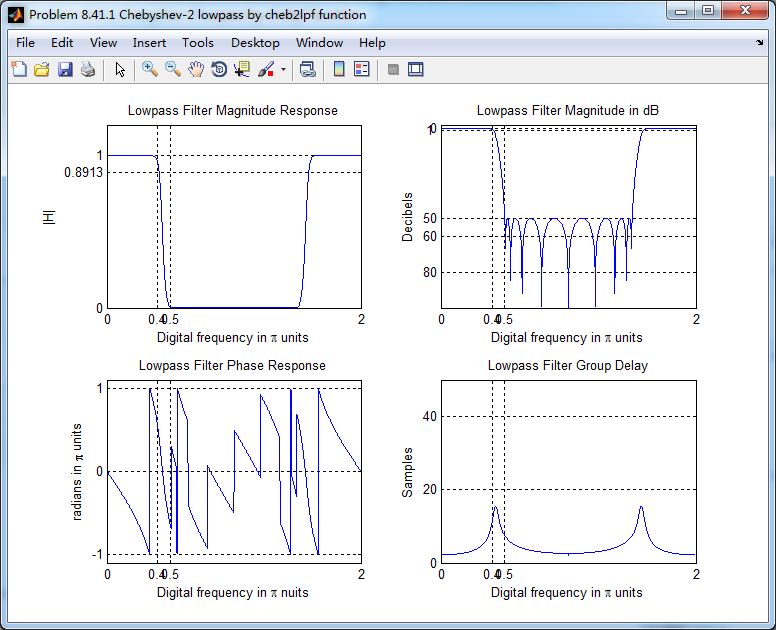
M = 2;                          % Omega max

subplot(2,2,1); plot(wwlp/pi, maglp); axis([0, M, 0, 1.2]); grid on;
xlabel('Digital frequency in \pi units'); ylabel('|H|'); title('Lowpass Filter Magnitude Response');
set(gca, 'XTickMode', 'manual', 'XTick', [0, 0.4, 0.5, M]);
set(gca, 'YTickMode', 'manual', 'YTick', [0, 0.8913, 1]);

subplot(2,2,2); plot(wwlp/pi, dblp); axis([0, M, -100, 2]); grid on;
xlabel('Digital frequency in \pi units'); ylabel('Decibels'); title('Lowpass Filter Magnitude in dB');
set(gca, 'XTickMode', 'manual', 'XTick', [0, 0.4, 0.5, M]);
set(gca, 'YTickMode', 'manual', 'YTick', [-80, -60, -50, -1, 0]);
set(gca,'YTickLabelMode','manual','YTickLabel',['80'; '60'; '50';'1 ';' 0']);

subplot(2,2,3); plot(wwlp/pi, phalp/pi); axis([0, M, -1.1, 1.1]); grid on;
xlabel('Digital frequency in \pi nuits'); ylabel('radians in \pi units'); title('Lowpass Filter Phase Response');
set(gca, 'XTickMode', 'manual', 'XTick', [0, 0.4, 0.5, M]);
set(gca, 'YTickMode', 'manual', 'YTick', [-1:1:1]);

subplot(2,2,4); plot(wwlp/pi, grdlp); axis([0, M, 0, 50]); grid on;
xlabel('Digital frequency in \pi units'); ylabel('Samples'); title('Lowpass Filter Group Delay');
set(gca, 'XTickMode', 'manual', 'XTick', [0, 0.4, 0.5, M]);
set(gca, 'YTickMode', 'manual', 'YTick', [0:20:50]);

% ------------------------------------------------------------
%                 PART 2   A/D and Reconstruction
% ------------------------------------------------------------

% Discrete time signal, Samples of analog signal xa(t)
Ts = 0.01;                       % sample intevel, second
Fs = 1/Ts;                       % sample frequency, Hz
n1_start = 0; n1_end = 500;
      n1 = [n1_start:1:n1_end];
     nTs = n1 * Ts;                   % [0, 5]s

xn1 = 3 * sin(40*pi*nTs) + 3 * cos(50*pi*nTs);    % digital signal

figure('NumberTitle', 'off', 'Name', 'Problem 8.41 xn1')
set(gcf,'Color','white');
subplot(2,1,1); stem(n1, xn1);
xlabel('n'); ylabel('x(n)');
title('xn sequence');  grid on;

% ----------------------------
%       DTFT of xn1
% ----------------------------
M = 500;
[X1, w] = dtft1(xn1, n1, M);

magX1  = abs(X1);  angX1  = angle(X1);  realX1  = real(X1);  imagX1  = imag(X1);

%% --------------------------------------------------------------------
%%              START X(w)'s  mag ang real imag
%% --------------------------------------------------------------------
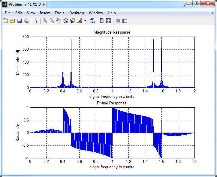
figure('NumberTitle', 'off', 'Name', 'Problem 8.41 X1 DTFT');
set(gcf,'Color','white');
subplot(2,1,1); plot(w/pi,magX1); grid on;  %axis([-1,1,0,1.05]);
title('Magnitude Response');
xlabel('digital frequency in \pi units'); ylabel('Magnitude  |H|');
subplot(2,1,2); plot(w/pi, angX1/pi); grid on;  %axis([-1,1,-1.05,1.05]);
title('Phase Response');
xlabel('digital frequency in \pi units'); ylabel('Radians/\pi');

figure('NumberTitle', 'off', 'Name', 'Problem 8.41 X1 DTFT');
set(gcf,'Color','white');
subplot(2,1,1); plot(w/pi, realX1); grid on;
title('Real Part');
xlabel('digital frequency in \pi units'); ylabel('Real');
subplot(2,1,2); plot(w/pi, imagX1); grid on;
title('Imaginary Part');
xlabel('digital frequency in \pi units'); ylabel('Imaginary');
%% -------------------------------------------------------------------
%%             END X's  mag ang real imag
%% -------------------------------------------------------------------

% -----------------------------------------
%       Reconstruction
%       methods: ZOH FOH spline  sinc
% -----------------------------------------
figure('NumberTitle', 'off', 'Name', 'Problem 8.41.2 Reconstruction xa(t) by ZOH');
set(gcf,'Color','white');
subplot(1,1,1); stairs(nTs*100, xn1); grid on;  %axis([0,1,0,1.5]);
title('Reconstructed Signal from x1(n) using Zero-Order-Hold function');
xlabel('t in msec units.'); ylabel('xa(n)'); hold on;
stem(nTs*100, xn1); gtext('Ts = 0.01 sec'); hold off;

figure('NumberTitle', 'off', 'Name', 'Problem 8.41.2 Reconstruction xa(t) by FOH');
set(gcf,'Color','white');
subplot(1,1,1); plot(nTs*100, xn1); grid on;  %axis([0,1,0,1.5]);
title('Reconstructed Signal from x1(n) using First-Order-Hold');
xlabel('t in msec units.'); ylabel('xa(n)'); hold on;
stem(nTs*100, xn1); gtext('Ts = 0.01 sec'); hold off;

% Reconstruction by spline function
Dt = 0.005; t = 0:Dt:5; xa = spline(nTs, xn1, t);
figure('NumberTitle', 'off', 'Name', sprintf('Problem 8.41.2 Reconstruction xa(t) by spline, Ts = %.4fs', Ts));
set(gcf,'Color','white');
%subplot(2,1,1);
plot(100*t, xa); xlabel('t in ms units'); ylabel('x');
title(sprintf('Reconstructed Signal from x1(n) using spline function')); grid on; hold on;
stem(100*nTs, xn1); gtext('spline');

%% --------------------------------------------------------------------
%%         Analog Signal reconstructed by sinc(x) function
%% --------------------------------------------------------------------

Dt = 0.005; t = 0:Dt:5;
xa = xn1 * sinc(Fs*(ones(length(n1),1)*t - nTs'*ones(1,length(t)))) ;

figure('NumberTitle', 'off', 'Name', 'Problem 8.41.2 Reconstruction by sinc function');
set(gcf,'Color','white');
subplot(1,1,1); plot(t*100, xa, 'r'); grid on;  %axis([0,1,0,1.5]);
title('Reconstructed Signal from x1(n) using sinc function');
xlabel('t in msec units.'); ylabel('xa(n)'); hold on;
stem(nTs*100, xn1, 'b', 'filled'); gtext('Ts=0.01 msec'); hold off;

% --------------------------------------------
%             PART 3:  Filter and D/A
% --------------------------------------------
yn1 = filter(blp, alp, xn1);

% ----------------------------
%       DTFT of yn1
% ----------------------------
M = 500;
[Y1, w] = dtft1(yn1, n1, M);

magY1  = abs(Y1);  angY1  = angle(Y1);  realY1  = real(Y1);  imagY1  = imag(Y1);

%% --------------------------------------------------------------------
%%              START Y1(w)'s  mag ang real imag
%% --------------------------------------------------------------------
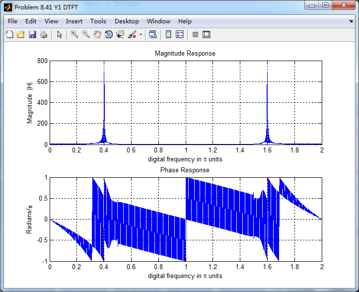
figure('NumberTitle', 'off', 'Name', 'Problem 8.41 Y1 DTFT');
set(gcf,'Color','white');
subplot(2,1,1); plot(w/pi,magY1); grid on;  %axis([-1,1,0,1.05]);
title('Magnitude Response');
xlabel('digital frequency in \pi units'); ylabel('Magnitude  |H|');
subplot(2,1,2); plot(w/pi, angY1/pi); grid on;  %axis([-1,1,-1.05,1.05]);
title('Phase Response');
xlabel('digital frequency in \pi units'); ylabel('Radians/\pi');

figure('NumberTitle', 'off', 'Name', 'Problem 8.41 Y1 DTFT');
set(gcf,'Color','white');
subplot(2,1,1); plot(w/pi, realY1); grid on;
title('Real Part');
xlabel('digital frequency in \pi units'); ylabel('Real');
subplot(2,1,2); plot(w/pi, imagY1); grid on;
title('Imaginary Part');
xlabel('digital frequency in \pi units'); ylabel('Imaginary');
%% -------------------------------------------------------------------
%%             END Y1's  mag ang real imag
%% -------------------------------------------------------------------

% -----------------------------------------
%       Reconstruction
%       methods: ZOH FOH spline  sinc
% -----------------------------------------
figure('NumberTitle', 'off', 'Name', 'Problem 8.41.2 Reconstruction ya(t) by ZOH');
set(gcf,'Color','white');
subplot(1,1,1); stairs(nTs*100, yn1); grid on;  %axis([0,1,0,1.5]);
title('Reconstructed Signal from y1(n) using Zero-Order-Hold function');
xlabel('t in msec units.'); ylabel('ya(n)'); hold on;
stem(nTs*100, yn1); gtext('Ts = 0.01 sec'); hold off;

figure('NumberTitle', 'off', 'Name', 'Problem 8.41.2 Reconstruction ya(t) by FOH');
set(gcf,'Color','white');
subplot(1,1,1); plot(nTs*100, yn1); grid on;  %axis([0,1,0,1.5]);
title('Reconstructed Signal from y1(n) using First-Order-Hold');
xlabel('t in msec units.'); ylabel('ya(n)'); hold on;
stem(nTs*100, yn1); gtext('Ts = 0.01 sec'); hold off;

% Reconstruction by spline function
Dt = 0.005; t = 0:Dt:5; ya = spline(nTs, yn1, t);
figure('NumberTitle', 'off', 'Name', sprintf('Problem 8.41.2 Reconstruction ya(t) by spline, Ts = %.4fs', Ts));
set(gcf,'Color','white');
%subplot(2,1,1);
plot(100*t, ya); xlabel('t in ms units'); ylabel('ya');
title(sprintf('Reconstructed Signal from y1(n) using spline function')); grid on; hold on;
stem(100*nTs, yn1); gtext('spline');

%% --------------------------------------------------------------------
%%         Analog Signal reconstructed by sinc(x) function
%% --------------------------------------------------------------------

Dt = 0.005; t = 0:Dt:5;
ya = yn1 * sinc(Fs*(ones(length(n1),1)*t - nTs'*ones(1,length(t)))) ;

figure('NumberTitle', 'off', 'Name', 'Problem 8.41.2 Reconstruction by sinc function');
set(gcf,'Color','white');
subplot(1,1,1); plot(t*100, ya, 'r'); grid on;  %axis([0,1,0,1.5]);
title('Reconstructed Signal from y1(n) using sinc function');
xlabel('t in msec units.'); ylabel('ya(n)'); hold on;
stem(nTs*100, yn1, 'b', 'filled'); gtext('Ts=0.01 msec'); hold off;

　　运行结果：

通带、阻带指标，绝对值单位

采用cheb2lpf函数，设计的Chebyshev-2型数字低通，系统函数串联形式系数

低通，幅度谱、相位谱和群延迟响应

采样信号的谱（DTFT变换），可看出，有两个数字频率分量，0.4π和0.5π

将采样信号通过设计的Chebyshev-2数字低通，得到输出y（n），其频谱如下，可看出，滤除了0.5π分量，仅保留0.4π分量

对离散信号y（n）采用sinc（插值函数）重建连续信号，如下图