《DSP using MATLAB》Problem 8.45

代码：

%% ------------------------------------------------------------------------
%%            Output Info about this m-file
fprintf('\n***********************************************************\n');
fprintf('        <DSP using MATLAB> Problem 8.45.4 \n\n');

banner();
%% ------------------------------------------------------------------------
%%
%%          Chebyshev-1 bandpass and lowpass, parallel form,
%%          by toolbox function in MATLAB,
%%
%% ------------------------------------------------------------------------

%--------------------------------------------------------
%           PART1 bandpass
% Digital Filter Specifications:   Chebyshev-1 bandpass
% -------------------------------------------------------
wsbp = [0.40*pi 0.90*pi];             % digital stopband freq in rad
wpbp = [0.60*pi 0.80*pi];             % digital passband freq in rad

delta1 = 0.05;
delta2 = 0.01;

Ripple = 0.5-delta1;                     % passband ripple in absolute
Attn = delta2;                           % stopband attenuation in absolute

  Rp = -20*log10(Ripple/0.5);             % passband ripple in dB
  As = -20*log10(Attn/0.5);               % stopband attenuation in dB

% Calculation of Chebyshev-1 filter parameters:
[N, wn] = cheb1ord(wpbp/pi, wsbp/pi, Rp, As);

fprintf('\n  ********* Chebyshev-1 Digital Bandpass Filter Order is = %3.0f \n', 2*N)

% Digital Chebyshev-1 Bandpass Filter Design:
[bbp, abp] = cheby1(N, Rp, wn);

[C, B, A] = dir2cas(0.5*bbp, abp)

% Calculation of Frequency Response:
[dbbp, magbp, phabp, grdbp, wwbp] = freqz_m(0.5*bbp, abp);

% -----------------------------------------------------
%    PART2  lowpass
% Digital Highpass Filter Specifications:
% -----------------------------------------------------
wslp = 0.40*pi;             % digital stopband freq in rad
wplp = 0.30*pi;             % digital passband freq in rad

delta1 = 0.10;
delta2 = 0.01;

Ripple = 1.0-delta1;                     % passband ripple in absolute
Attn = delta2;                           % stopband attenuation in absolute

  Rp = -20*log10(Ripple/1.0);             % passband ripple in dB
  As = -20*log10(Attn/1.0);               % stopband attenuation in dB

% Calculation of Chebyshev-1 filter parameters:
[N, wn] = cheb1ord(wplp/pi, wslp/pi, Rp, As);

fprintf('\n  ********* Chebyshev-1 Digital Lowpass Filter Order is = %3.0f \n', N)

% Digital Chebyshev-1 lowpass Filter Design:
[blp, alp] = cheby1(N, Rp, wn);

[C, B, A] = dir2cas(blp, alp)

% Calculation of Frequency Response:
[dblp, maglp, phalp, grdlp, wwlp] = freqz_m(blp, alp);

% ---------------------------------------------
%      PART3   parallel form of bp and lp
% ---------------------------------------------
abp;
bbp;
alp;
blp;

fprintf('\n  ********* Chebyshev-1 Digital Lowpass parrell with Bandpass Filter *******\n');
fprintf('\n  ********* Coefficients of Direct-Form: *******\n');
a = conv(2*abp, alp)
b = conv(bbp, alp) + conv(blp, 2*abp)
[C, B, A] = dir2cas(b, a)

% Calculation of Frequency Response:
[db, mag, pha, grd, ww] = freqz_m(b, a);

%% -----------------------------------------------------------------
%%                             Plot
%% -----------------------------------------------------------------  

figure('NumberTitle', 'off', 'Name', 'Problem 8.45.4 combination of Chebyshev-1 bp and lp, by cheby1 function in MATLAB')
set(gcf,'Color','white');
M = 1;                          % Omega max

subplot(2,2,1); plot(ww/pi, mag); axis([0, M, 0, 1.2]); grid on;
xlabel('Digital frequency in \pi units'); ylabel('|H|'); title('Magnitude Response');
set(gca, 'XTickMode', 'manual', 'XTick', [0, wplp/pi, wsbp(1)/pi, wpbp/pi, wsbp(2)/pi, M]);
set(gca, 'YTickMode', 'manual', 'YTick', [0, 0.01, 0.45, 0.5, 0.9, 1]);

subplot(2,2,2); plot(ww/pi, db); axis([0, M, -100, 2]); grid on;
xlabel('Digital frequency in \pi units'); ylabel('Decibels'); title('Magnitude in dB');
set(gca, 'XTickMode', 'manual', 'XTick', [0, wplp/pi, wsbp(1)/pi, wpbp/pi, wsbp(2)/pi, M]);
set(gca, 'YTickMode', 'manual', 'YTick', [-76, -46, -41, -1, 0]);
set(gca,'YTickLabelMode','manual','YTickLabel',['76'; '46'; '41';'1 ';' 0']);

subplot(2,2,3); plot(ww/pi, pha/pi); axis([0, M, -1.1, 1.1]); grid on;
xlabel('Digital frequency in \pi nuits'); ylabel('radians in \pi units'); title('Phase Response');
set(gca, 'XTickMode', 'manual', 'XTick', [0, wplp/pi, wsbp(1)/pi, wpbp/pi, wsbp(2)/pi, M]);
set(gca, 'YTickMode', 'manual', 'YTick', [-1:0.5:1]);

subplot(2,2,4); plot(ww/pi, grd); axis([0, M, 0, 80]); grid on;
xlabel('Digital frequency in \pi units'); ylabel('Samples'); title('Group Delay');
set(gca, 'XTickMode', 'manual', 'XTick', [0, wplp/pi, wsbp(1)/pi, wpbp/pi, wsbp(2)/pi, M]);
set(gca, 'YTickMode', 'manual', 'YTick', [0:20:80]);

figure('NumberTitle', 'off', 'Name', 'Problem 8.45.4 combination of Chebyshev-1 bp and lp, by cheby1')
set(gcf,'Color','white');
M = 1;                          % Omega max

%subplot(2,2,1);
plot(ww/pi, mag); axis([0, M, 0, 1.2]); grid on;
xlabel('Digital frequency in \pi units'); ylabel('|H|'); title('Magnitude Response');
set(gca, 'XTickMode', 'manual', 'XTick', [0, wplp/pi, wsbp(1)/pi, wpbp/pi, wsbp(2)/pi, M]);
set(gca, 'YTickMode', 'manual', 'YTick', [0, 0.01, 0.45, 0.5, 0.9, 1]);

figure('NumberTitle', 'off', 'Name', 'Problem 8.45.4 Pole-Zero Plot')
set(gcf,'Color','white');
zplane(b, a);
title(sprintf('Pole-Zero Plot'));
%pzplotz(b,a);

　　运行结果：

看题目设计要求，是Chebyshev-1型低通和带通的组合。

我们先设计带通，系统函数串联形式的系数如下：

其次，Chebyshev-1型数字低通，阶数为7，系统函数串联形式的系数如下：

再次，低通和带通进行组合，等效滤波器的系统函数，直接形式和串联形式，系数分别如下：

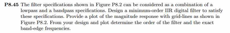
等效滤波器，幅度谱如下，频带边界频率和指标画出直线，

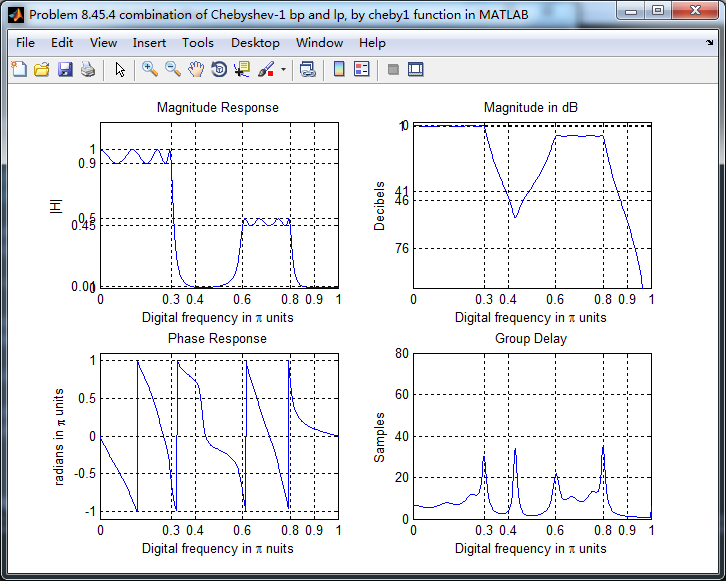
幅度谱、相位谱和群延迟响应

零极点图