《DSP using MATLAB》Problem 8.9

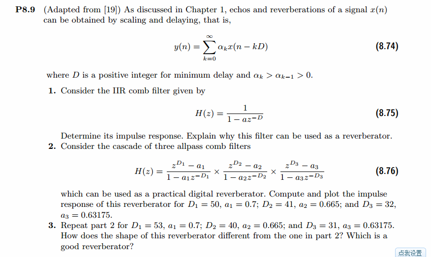
代码：

%% ------------------------------------------------------------------------
%%            Output Info about this m-file
fprintf('\n***********************************************************\n');
fprintf('        <DSP using MATLAB> Problem 8.9 \n\n');
banner();
%% ------------------------------------------------------------------------

a0 = -0.9;
% digital iir lowpass filter
b = [1 ];
a = [1 a0];

figure('NumberTitle', 'off', 'Name', 'Problem 8.9 Pole-Zero Plot')
set(gcf,'Color','white');
zplane(b,a);
title(sprintf('Pole-Zero Plot'));
%pzplotz(b,a);

% corresponding system function  Direct form
K = 1;                                                                     % gain parameter
b = K*b;                                                                    % denominator
a = a;                                                                      % numerator

[db, mag, pha, grd, w] = freqz_m(b, a);

% ---------------------------------------------------------------------
%  Choose the gain parameter of the filter, maximum gain is equal to 1
% ---------------------------------------------------------------------
gain1=max(mag)                    % with poles
K = 1/gain1
[db, mag, pha, grd, w] = freqz_m(K*b, a);

figure('NumberTitle', 'off', 'Name', 'Problem 8.9 IIR lowpass filter')
set(gcf,'Color','white'); 

subplot(2,2,1); plot(w/pi, db); grid on; axis([0 2 -60 10]);
set(gca,'YTickMode','manual','YTick',[-60,-30,0])
set(gca,'YTickLabelMode','manual','YTickLabel',['60';'30';' 0']);
set(gca,'XTickMode','manual','XTick',[0,0.25,0.5,1,1.5,1.75,2]);
xlabel('frequency in \pi units'); ylabel('Decibels'); title('Magnitude Response in dB');

subplot(2,2,3); plot(w/pi, mag); grid on; %axis([0 1 -100 10]);
xlabel('frequency in \pi units'); ylabel('Absolute'); title('Magnitude Response in absolute');
set(gca,'XTickMode','manual','XTick',[0,0.25,0.5,1,1.5,1.75,2]);
set(gca,'YTickMode','manual','YTick',[0,1.0]);

subplot(2,2,2); plot(w/pi, pha); grid on; %axis([0 1 -100 10]);
xlabel('frequency in \pi units'); ylabel('Rad'); title('Phase Response in Radians');

subplot(2,2,4); plot(w/pi, grd*pi/180);  grid on; %axis([0 1 -100 10]);
xlabel('frequency in \pi units'); ylabel('Rad'); title('Group Delay');
set(gca,'XTickMode','manual','XTick',[0,0.25,0.5,1,1.5,1.75,2]);
%set(gca,'YTickMode','manual','YTick',[0,1.0]);

% Impulse Response
fprintf('\n----------------------------------');
fprintf('\nPartial fraction expansion method: \n');
[R, p, c] = residuez(K*b,a)
MR = (abs(R))'              % Residue  Magnitude
AR = (angle(R))'/pi         % Residue  angles in pi units
Mp = (abs(p))'              % pole  Magnitude
Ap = (angle(p))'/pi         % pole  angles in pi units
[delta, n] = impseq(0,0,50);
h_chk = filter(K*b,a,delta);      % check sequences

% ------------------------------------------------------------------------------------------------
%                                gain parameter K
% ------------------------------------------------------------------------------------------------
h =  ( 0.9.^n ) .* (0.1000) + 0 * delta;
% ------------------------------------------------------------------------------------------------

figure('NumberTitle', 'off', 'Name', 'Problem 8.9 IIR lp filter, h(n) by filter and Inv-Z ')
set(gcf,'Color','white'); 

subplot(2,1,1); stem(n, h_chk); grid on; %axis([0 2 -60 10]);
xlabel('n'); ylabel('h\_chk'); title('Impulse Response sequences by filter');

subplot(2,1,2); stem(n, h); grid on; %axis([0 1 -100 10]);
xlabel('n'); ylabel('h'); title('Impulse Response sequences by Inv-Z');

[db, mag, pha, grd, w] = freqz_m(h, [1]);

figure('NumberTitle', 'off', 'Name', 'Problem 8.9 IIR filter, h(n) by Inv-Z ')
set(gcf,'Color','white'); 

subplot(2,2,1); plot(w/pi, db); grid on; axis([0 2 -60 10]);
set(gca,'YTickMode','manual','YTick',[-60,-30,0])
set(gca,'YTickLabelMode','manual','YTickLabel',['60';'30';' 0']);
set(gca,'XTickMode','manual','XTick',[0,0.25,1,1.75,2]);
xlabel('frequency in \pi units'); ylabel('Decibels'); title('Magnitude Response in dB');

subplot(2,2,3); plot(w/pi, mag); grid on; %axis([0 1 -100 10]);
xlabel('frequency in \pi units'); ylabel('Absolute'); title('Magnitude Response in absolute');
set(gca,'XTickMode','manual','XTick',[0,0.25,1,1.75,2]);
set(gca,'YTickMode','manual','YTick',[0,1.0]);

subplot(2,2,2); plot(w/pi, pha); grid on; %axis([0 1 -100 10]);
xlabel('frequency in \pi units'); ylabel('Rad'); title('Phase Response in Radians');

subplot(2,2,4); plot(w/pi, grd*pi/180);  grid on; %axis([0 1 -100 10]);
xlabel('frequency in \pi units'); ylabel('Rad'); title('Group Delay');
set(gca,'XTickMode','manual','XTick',[0,0.25,1,1.75,2]);
%set(gca,'YTickMode','manual','YTick',[0,1.0]);

% --------------------------------------------------
%               digital IIR comb filter
%           system function  Direct form
% --------------------------------------------------
D = 4;
b = K*[1];
a = [1  zeros(1,D-1)  a0];

figure('NumberTitle', 'off', 'Name', 'Problem 8.9 Pole-Zero Plot')
set(gcf,'Color','white');
zplane(b,a);
title(sprintf('Pole-Zero Plot'));

[db, mag, pha, grd, w] = freqz_m(b, a);

figure('NumberTitle', 'off', 'Name', 'Problem 8.9 IIR comb filter')
set(gcf,'Color','white'); 

subplot(2,2,1); plot(w/pi, db); grid on; axis([0 2 -60 10]);
set(gca,'YTickMode','manual','YTick',[-60,-30,0])
set(gca,'YTickLabelMode','manual','YTickLabel',['60';'30';' 0']);
set(gca,'XTickMode','manual','XTick',[0,0.25,0.5,1,1.5,1.75,2]);
xlabel('frequency in \pi units'); ylabel('Decibels'); title('Magnitude Response in dB');

subplot(2,2,3); plot(w/pi, mag); grid on; %axis([0 1 -100 10]);
xlabel('frequency in \pi units'); ylabel('Absolute'); title('Magnitude Response in absolute');
set(gca,'XTickMode','manual','XTick',[0,0.25,0.5,1,1.5,1.75,2]);
set(gca,'YTickMode','manual','YTick',[0,1.0]);

subplot(2,2,2); plot(w/pi, pha); grid on; %axis([0 1 -100 10]);
xlabel('frequency in \pi units'); ylabel('Rad'); title('Phase Response in Radians');

subplot(2,2,4); plot(w/pi, grd*pi/180);  grid on; %axis([0 1 -100 10]);
xlabel('frequency in \pi units'); ylabel('Rad'); title('Group Delay');
set(gca,'XTickMode','manual','XTick',[0,0.25,0.5,1,1.5,1.75,2]);
%set(gca,'YTickMode','manual','YTick',[0,1.0]);

% Impulse Response
fprintf('\n----------------------------------');
fprintf('\nPartial fraction expansion method: \n');
[R, p, c] = residuez(b,a)
MR = (abs(R))'              % Residue  Magnitude
AR = (angle(R))'/pi         % Residue  angles in pi units
Mp = (abs(p))'              % pole  Magnitude
Ap = (angle(p))'/pi         % pole  angles in pi units
[delta, n] = impseq(0,0,200);
h_chk = filter(b,a,delta);      % check sequences

% ------------------------------------------------------------------------------------------------
%                                gain parameter K
% ------------------------------------------------------------------------------------------------
h =  0.0250 * ( ( 0.9740.^n ) .* ( 2*cos(pi*n/2) + (-1).^n + 1) ) + 0.0*delta;
% ------------------------------------------------------------------------------------------------

figure('NumberTitle', 'off', 'Name', 'Problem 8.9 Comb filter, h(n) by filter and Inv-Z ')
set(gcf,'Color','white'); 

subplot(2,1,1); stem(n, h_chk); grid on; %axis([0 2 -60 10]);
xlabel('n'); ylabel('h\_chk'); title('Impulse Response sequences by filter');

subplot(2,1,2); stem(n, h); grid on; %axis([0 1 -100 10]);
xlabel('n'); ylabel('h'); title('Impulse Response sequences by Inv-Z');

[db, mag, pha, grd, w] = freqz_m(h, [1]);

figure('NumberTitle', 'off', 'Name', 'Problem 8.9 Comb filter, h(n) by Inv-Z ')
set(gcf,'Color','white'); 

subplot(2,2,1); plot(w/pi, db); grid on; axis([0 2 -60 10]);
set(gca,'YTickMode','manual','YTick',[-60,-30,0])
set(gca,'YTickLabelMode','manual','YTickLabel',['60';'30';' 0']);
set(gca,'XTickMode','manual','XTick',[0,0.25,1,1.75,2]);
xlabel('frequency in \pi units'); ylabel('Decibels'); title('Magnitude Response in dB');

subplot(2,2,3); plot(w/pi, mag); grid on; %axis([0 1 -100 10]);
xlabel('frequency in \pi units'); ylabel('Absolute'); title('Magnitude Response in absolute');
set(gca,'XTickMode','manual','XTick',[0,0.25,1,1.75,2]);
set(gca,'YTickMode','manual','YTick',[0,1.0]);

subplot(2,2,2); plot(w/pi, pha); grid on; %axis([0 1 -100 10]);
xlabel('frequency in \pi units'); ylabel('Rad'); title('Phase Response in Radians');

subplot(2,2,4); plot(w/pi, grd*pi/180);  grid on; %axis([0 1 -100 10]);
xlabel('frequency in \pi units'); ylabel('Rad'); title('Group Delay');
set(gca,'XTickMode','manual','XTick',[0,0.25,1,1.75,2]);
%set(gca,'YTickMode','manual','YTick',[0,1.0]);

　　运行结果：

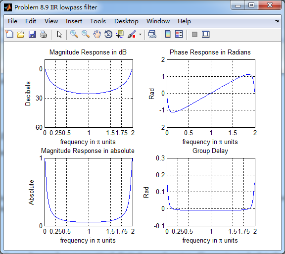
D=1，单个滤波器

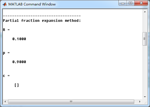
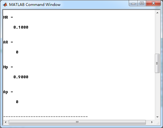
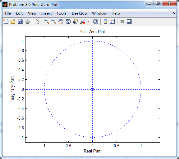
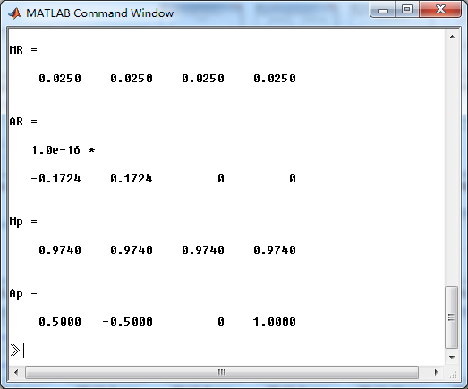
这里取D=4，单个重复4次，系统函数部分分式展开，

第2、3小题不会。