《DSP using MATLAB》Problem 8.7

代码：

%% ------------------------------------------------------------------------

%%            Output Info about this m-file

fprintf('\n***********************************************************\n');

fprintf('        <DSP using MATLAB> Problem 8.7 \n\n');

banner();

%% ------------------------------------------------------------------------

% digital iir lowpass filter

b = [1 1];

a = [1 -0.9];

figure('NumberTitle', 'off', 'Name', 'Problem 8.7 Pole-Zero Plot')

set(gcf,'Color','white');

zplane(b,a);

title(sprintf('Pole-Zero Plot'));

%pzplotz(b,a);

% corresponding system function  Direct form

K = 1;                                                                     % gain parameter

b = K*b;                                                                    % denominator

a = a;                                                                      % numerator

[db, mag, pha, grd, w] = freqz_m(b, a);

% ---------------------------------------------------------------------

%  Choose the gain parameter of the filter, maximum gain is equal to 1

% ---------------------------------------------------------------------

gain1=max(mag)                    % with poles

K = 1/gain1

[db, mag, pha, grd, w] = freqz_m(K*b, a);

figure('NumberTitle', 'off', 'Name', 'Problem 8.7 IIR lowpass filter')

set(gcf,'Color','white'); 

subplot(2,2,1); plot(w/pi, db); grid on; axis([0 2 -60 10]);

set(gca,'YTickMode','manual','YTick',[-60,-30,0])

set(gca,'YTickLabelMode','manual','YTickLabel',['60';'30';' 0']);

set(gca,'XTickMode','manual','XTick',[0,0.25,0.5,1,1.5,1.75,2]);

xlabel('frequency in \pi units'); ylabel('Decibels'); title('Magnitude Response in dB');

subplot(2,2,3); plot(w/pi, mag); grid on; %axis([0 1 -100 10]);

xlabel('frequency in \pi units'); ylabel('Absolute'); title('Magnitude Response in absolute');

set(gca,'XTickMode','manual','XTick',[0,0.25,0.5,1,1.5,1.75,2]);

set(gca,'YTickMode','manual','YTick',[0,1.0]);

subplot(2,2,2); plot(w/pi, pha); grid on; %axis([0 1 -100 10]);

xlabel('frequency in \pi units'); ylabel('Rad'); title('Phase Response in Radians');

subplot(2,2,4); plot(w/pi, grd*pi/180);  grid on; %axis([0 1 -100 10]);

xlabel('frequency in \pi units'); ylabel('Rad'); title('Group Delay');

set(gca,'XTickMode','manual','XTick',[0,0.25,0.5,1,1.5,1.75,2]);

%set(gca,'YTickMode','manual','YTick',[0,1.0]);

% Impulse Response

fprintf('\n----------------------------------');

fprintf('\nPartial fraction expansion method: \n');

[R, p, c] = residuez(b,a)

MR = (abs(R))'              % Residue  Magnitude

AR = (angle(R))'/pi         % Residue  angles in pi units

Mp = (abs(p))'              % pole  Magnitude

Ap = (angle(p))'/pi         % pole  angles in pi units

[delta, n] = impseq(0,0,50);

h_chk = filter(b,a,delta);      % check sequences

% ------------------------------------------------------------------------------------------------

%                                gain parameter K=0.05

% ------------------------------------------------------------------------------------------------

h =  ( 0.9.^n ) .* 0.1056 - 0.0556 * delta;

% ------------------------------------------------------------------------------------------------

figure('NumberTitle', 'off', 'Name', 'Problem 8.7 IIR lp filter, h(n) by filter and Inv-Z ')

set(gcf,'Color','white'); 

subplot(2,1,1); stem(n, h_chk); grid on; %axis([0 2 -60 10]);

xlabel('n'); ylabel('h\_chk'); title('Impulse Response sequences by filter');

subplot(2,1,2); stem(n, h); grid on; %axis([0 1 -100 10]);

xlabel('n'); ylabel('h'); title('Impulse Response sequences by Inv-Z');

[db, mag, pha, grd, w] = freqz_m(h, [1]);

figure('NumberTitle', 'off', 'Name', 'Problem 8.7 IIR filter, h(n) by Inv-Z ')

set(gcf,'Color','white'); 

subplot(2,2,1); plot(w/pi, db); grid on; axis([0 2 -60 10]);

set(gca,'YTickMode','manual','YTick',[-60,-30,0])

set(gca,'YTickLabelMode','manual','YTickLabel',['60';'30';' 0']);

set(gca,'XTickMode','manual','XTick',[0,0.25,1,1.75,2]);

xlabel('frequency in \pi units'); ylabel('Decibels'); title('Magnitude Response in dB');

subplot(2,2,3); plot(w/pi, mag); grid on; %axis([0 1 -100 10]);

xlabel('frequency in \pi units'); ylabel('Absolute'); title('Magnitude Response in absolute');

set(gca,'XTickMode','manual','XTick',[0,0.25,1,1.75,2]);

set(gca,'YTickMode','manual','YTick',[0,1.0]);

subplot(2,2,2); plot(w/pi, pha); grid on; %axis([0 1 -100 10]);

xlabel('frequency in \pi units'); ylabel('Rad'); title('Phase Response in Radians');

subplot(2,2,4); plot(w/pi, grd*pi/180);  grid on; %axis([0 1 -100 10]);

xlabel('frequency in \pi units'); ylabel('Rad'); title('Group Delay');

set(gca,'XTickMode','manual','XTick',[0,0.25,1,1.75,2]);

%set(gca,'YTickMode','manual','YTick',[0,1.0]);

% --------------------------------------------------

%               digital IIR comb filter

% --------------------------------------------------

b = K*[1  0  0  0  0  0  1];

a = [1  0  0  0  0  0  -0.9];

figure('NumberTitle', 'off', 'Name', 'Problem 8.7 Pole-Zero Plot')

set(gcf,'Color','white');

zplane(b,a);

title(sprintf('Pole-Zero Plot'));

[db, mag, pha, grd, w] = freqz_m(b, a);

figure('NumberTitle', 'off', 'Name', 'Problem 8.7 IIR comb filter')

set(gcf,'Color','white'); 

subplot(2,2,1); plot(w/pi, db); grid on; axis([0 2 -60 10]);

set(gca,'YTickMode','manual','YTick',[-60,-30,0])

set(gca,'YTickLabelMode','manual','YTickLabel',['60';'30';' 0']);

set(gca,'XTickMode','manual','XTick',[0,0.25,0.5,1,1.5,1.75,2]);

xlabel('frequency in \pi units'); ylabel('Decibels'); title('Magnitude Response in dB');

subplot(2,2,3); plot(w/pi, mag); grid on; %axis([0 1 -100 10]);

xlabel('frequency in \pi units'); ylabel('Absolute'); title('Magnitude Response in absolute');

set(gca,'XTickMode','manual','XTick',[0,0.25,0.5,1,1.5,1.75,2]);

set(gca,'YTickMode','manual','YTick',[0,1.0]);

subplot(2,2,2); plot(w/pi, pha); grid on; %axis([0 1 -100 10]);

xlabel('frequency in \pi units'); ylabel('Rad'); title('Phase Response in Radians');

subplot(2,2,4); plot(w/pi, grd*pi/180);  grid on; %axis([0 1 -100 10]);

xlabel('frequency in \pi units'); ylabel('Rad'); title('Group Delay');

set(gca,'XTickMode','manual','XTick',[0,0.25,0.5,1,1.5,1.75,2]);

%set(gca,'YTickMode','manual','YTick',[0,1.0]);

% Impulse Response

fprintf('\n----------------------------------');

fprintf('\nPartial fraction expansion method: \n');

[R, p, c] = residuez(b,a)

MR = (abs(R))'              % Residue  Magnitude

AR = (angle(R))'/pi         % Residue  angles in pi units

Mp = (abs(p))'              % pole  Magnitude

Ap = (angle(p))'/pi         % pole  angles in pi units

[delta, n] = impseq(0,0,300);

h_chk = filter(b,a,delta);      % check sequences

% ------------------------------------------------------------------------------------------------

%                                gain parameter K=0.05

% ------------------------------------------------------------------------------------------------

%h =  0.0211 * (( 0.9791.^n ) .* (2*cos(0.4*pi*n) + 2*cos(0.8*pi*n) + 1)) - 0.0556*delta;  %L=5;

h =  0.0176 * ( ( 0.9826.^n ) .* ( 2*cos(2*pi*n/3) + 2*cos(pi*n/3) + (-1).^n + 1) ) - 0.0556*delta;  %L=6;

% ------------------------------------------------------------------------------------------------

figure('NumberTitle', 'off', 'Name', 'Problem 8.7 Comb filter, h(n) by filter and Inv-Z ')

set(gcf,'Color','white'); 

subplot(2,1,1); stem(n, h_chk); grid on; %axis([0 2 -60 10]);

xlabel('n'); ylabel('h\_chk'); title('Impulse Response sequences by filter');

subplot(2,1,2); stem(n, h); grid on; %axis([0 1 -100 10]);

xlabel('n'); ylabel('h'); title('Impulse Response sequences by Inv-Z');

[db, mag, pha, grd, w] = freqz_m(h, [1]);

figure('NumberTitle', 'off', 'Name', 'Problem 8.7 Comb filter, h(n) by Inv-Z ')

set(gcf,'Color','white'); 

subplot(2,2,1); plot(w/pi, db); grid on; axis([0 2 -60 10]);

set(gca,'YTickMode','manual','YTick',[-60,-30,0])

set(gca,'YTickLabelMode','manual','YTickLabel',['60';'30';' 0']);

set(gca,'XTickMode','manual','XTick',[0,0.25,1,1.75,2]);

xlabel('frequency in \pi units'); ylabel('Decibels'); title('Magnitude Response in dB');

subplot(2,2,3); plot(w/pi, mag); grid on; %axis([0 1 -100 10]);

xlabel('frequency in \pi units'); ylabel('Absolute'); title('Magnitude Response in absolute');

set(gca,'XTickMode','manual','XTick',[0,0.25,1,1.75,2]);

set(gca,'YTickMode','manual','YTick',[0,1.0]);

subplot(2,2,2); plot(w/pi, pha); grid on; %axis([0 1 -100 10]);

xlabel('frequency in \pi units'); ylabel('Rad'); title('Phase Response in Radians');

subplot(2,2,4); plot(w/pi, grd*pi/180);  grid on; %axis([0 1 -100 10]);

xlabel('frequency in \pi units'); ylabel('Rad'); title('Group Delay');

set(gca,'XTickMode','manual','XTick',[0,0.25,1,1.75,2]);

%set(gca,'YTickMode','manual','YTick',[0,1.0]);

　　运行结果：

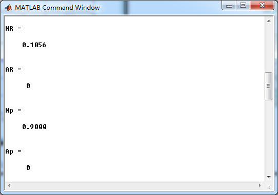
先计算单个IIR低通，

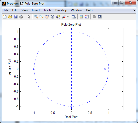
零极点

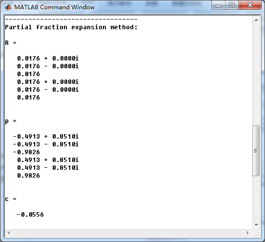
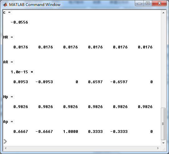
L=6阶梳状低通，系统函数部分分式展开如下

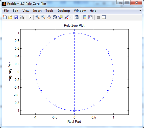
梳状低通滤波器零极点图

幅度谱、相位谱、群延迟

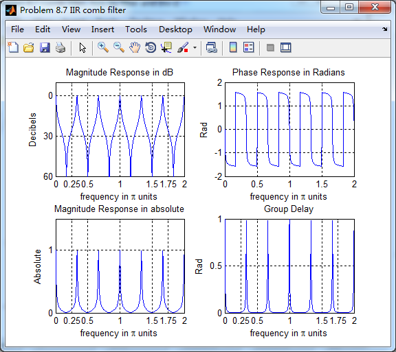
可以看出，在0到2π范围内，单个低通重复出现了6次，原来的谱压缩到六分之一。

《DSP using MATLAB》Problem 8.7的更多相关文章

《DSP using MATLAB》Problem 7.27
代码: %% ++++++++++++++++++++++++++++++++++++++++++++++++++++++++++++++++++++++++++++++++ %% Output In ...
《DSP using MATLAB》Problem 7.26
注意:高通的线性相位FIR滤波器,不能是第2类,所以其长度必须为奇数.这里取M=31,过渡带里采样值抄书上的. 代码: %% +++++++++++++++++++++++++++++++++++++ ...
《DSP using MATLAB》Problem 7.25
代码: %% ++++++++++++++++++++++++++++++++++++++++++++++++++++++++++++++++++++++++++++++++ %% Output In ...
《DSP using MATLAB》Problem 7.24
又到清明时节,…… 注意:带阻滤波器不能用第2类线性相位滤波器实现,我们采用第1类,长度为基数,选M=61 代码: %% +++++++++++++++++++++++++++++++++++++++ ...
《DSP using MATLAB》Problem 7.23
%% ++++++++++++++++++++++++++++++++++++++++++++++++++++++++++++++++++++++++++++++++ %% Output Info a ...
《DSP using MATLAB》Problem 7.16
使用一种固定窗函数法设计带通滤波器. 代码: %% ++++++++++++++++++++++++++++++++++++++++++++++++++++++++++++++++++++++++++ ...
《DSP using MATLAB》Problem 7.15
用Kaiser窗方法设计一个台阶状滤波器. 代码: %% +++++++++++++++++++++++++++++++++++++++++++++++++++++++++++++++++++++++ ...
《DSP using MATLAB》Problem 7.14
代码: %% ++++++++++++++++++++++++++++++++++++++++++++++++++++++++++++++++++++++++++++++++ %% Output In ...
《DSP using MATLAB》Problem 7.13
代码: %% ++++++++++++++++++++++++++++++++++++++++++++++++++++++++++++++++++++++++++++++++ %% Output In ...
《DSP using MATLAB》Problem 7.12
阻带衰减50dB,我们选Hamming窗代码: %% ++++++++++++++++++++++++++++++++++++++++++++++++++++++++++++++++++++++++ ...

随机推荐

js倒计时在移动端的应用
在移动端测试倒计时,将时间转化为毫秒会在苹果手机上出现NaN ``` //在安卓上这样写可以获取到的 var date = '2017-06-12 13:12:13'; var time = new ...
shell 命令文件查看ls，复制cp，移动mv，查看文件内容cat more less，查看文件信息 file
1. 查看文件 ls ls -l 查看文件详细信息 ls -a 查看所有文件(包含隐藏文件) ls -lh 带单位显示文件大小 ls -i 查看文件的节点号(相当身份证唯一) 2 ...
matplotlib实现伪彩色图像和色度条的展现
灰度图显示为伪彩色图法一 import matplotlib.pyplot as plt img = plt.imread('C:/Users/leex/Desktop/lena.jpg') img ...
校园商铺-2项目设计和框架搭建-7验证Dao
以最简单的地区表为例 1.插入数据 insert into tb_area (area_name, priority) values('东苑', 1),('南苑', 7),('北苑', 5); sel ...
java反射获取和设置实体类的属性值递归所有父类
最近做一个通用数据操作接口,需要动态获取和设置实体类的属性值,为了通用实体做了多重继承,开始网上找到代码都不支持父类操作,只能自己搞一个工具类了,此工具类可以设置和获取所有父类属性,代码贴下面拿走不谢 ...
关于web前端网站优化
不知道是哪位大牛的文章,转过来嘻嘻. 作者:斯迪链接:https://www.zhihu.com/question/21658448/answer/18903129来源:知乎著作权归作者所有.商业转载 ...
[BJOI 2018]染色
题意:求01成立. 并查集维护,记录一个变量判断决策. #include<bits/stdc++.h> using namespace std; #define int long long ...
.NETFramework：template
ylbtech-.NETFramework: 1.返回顶部 2.返回顶部 3.返回顶部 4.返回顶部 5.返回顶部 6.返回顶部作者:ylbtech出处:http://y ...
transient在java中的作用
java 的transient关键字的作用是需要实现Serilizable接口,将不需要序列化的属性前添加关键字transient,序列化对象的时候,这个属性就不会序列化到指定的目的地中. trans ...
PAT甲级——A1107 Social Clusters
When register on a social network, you are always asked to specify your hobbies in order to find som ...

《DSP using MATLAB》Problem 8.7

《DSP using MATLAB》Problem 8.7的更多相关文章

随机推荐

热门专题